Chapter 15 Ensemble Methods
Reference: Ch8 in An introduction to Statistical Learning with applications in R by James, Witten, Hastie and Tibshirani. For more details, study STAT457/ 462.
Package used:
Ensemble methods involve pooling together the predictions of a set of many models.
In this chapter, we illustrate this idea by pooling together many decision trees, resulting in a method called random forest. Another powerful technique is called boosting.
However, it is important to note that ensemble method is a generally method that can be applied not only to tree-based methods but virtually any models. For example, you can combine the predictions from a neural network and a random forest. In fact, many of the winners of the machine-learning competitions on Kaggle use very large ensembles of models.
Remark: of course, to get a good performance, the weights used to combine the models should be optimized on the validation data.
The main idea of ensemble methods is to combine models that are as good as possible while being as different as possible.
Analogy: combining experts from different fields to solve a difficult problem is usually more effective than one single expert or a group of experts in the same field.
15.1 Bagging
Bagging = Bootstrap aggregation
- a general-purpose procedure for reducing the variance of a statistical learning method
Suppose we can compute a prediction \(\hat{f}(x)\) given data \(\{(x_i, y_i)\}^n_{i=1}\).
Bagging steps:
Sample with replacement \(n\) data from \(\{(x_i, y_i)\}^n_{i=1}\). Denote the resampled data to be \(\{(x^{(b)}_i, y^{(b)}_i)\}^n_{i=1}\).
Compute \(\hat{f}^{(b)}(x)\) using \(\{(x^{(b)}_i, y^{(b)}_i)\}^n_{i=1}\).
Repeat Step 1-2 \(B\) times to obtain \(\hat{f}^{(b)}(x)\) for \(b =1,\ldots,B\).
Final model is \[\begin{equation*} \hat{f}_{Bagging}(x) = \frac{1}{B} \sum^B_{i=1} \hat{f}^{(b)}(x). \end{equation*}\]
15.2 Random Forest
Bagging decision trees uses the same model and variables repeatedly. Thus, the models lack diversity. In fact, the bagged trees are highly correlated. To improve the prediction accuracy, we want to combine trees that are “different”.
Random forest includes a small tweak that decorrelates the trees used in the ensemble.
Ideas of random forest:
As in bagging, a number of decision trees are build on boostrapped training samples.
But when building these decision trees, each time a split in a tree is considered, only a random sample of \(m\) predictors is chosen as split candidates from the full set of \(p\) predictors.
A fresh sample of \(m\) predictors is taken each split.
In this way, the correlation between the predictions from the trees will be reduced because each tree is built using only a subset of predictors at each split.
Remark: when \(m = p\), random forest is the same as bagging decision tree.
15.2.1 Example
We will use the Hitters dataset from the package ISLR2 to illustrate how to perform random forest with the function randomForest() in the package randomForest.
Hitters <- na.omit(Hitters)

# split the dataset
set.seed(1)
index <- sample(nrow(Hitters), nrow(Hitters) * 0.5)
Hitters_train <- Hitters[index, ]
Hitters_test <- Hitters[-index, ]
Fitting a random forest:
rf_fit <- randomForest(Salary ~., data = Hitters_train,
                       mtry = (ncol(Hitters_train) - 1)/ 3, ntree = 1000, importance = TRUE)
Two important parameters:
mtry: Number of variables randomly sampled as candidates at each split. The default values for classification and regression are \(\sqrt{p}\) and \(p/3\), respectively.
ntree: Number of trees to grow. The default is \(500\). More trees will require more time.
Prediction:
# Obtain prediction on test data
rf_pred <- predict(rf_fit, Hitters_test)

# Compute MSE in test data
mean((Hitters_test$Salary - rf_pred)^2)
## [1] 87650.31
Compared with a multiple linear regression model:
# Fit linear regression model
ls_fit <- lm(Salary ~., data = Hitters_train)

# Obtain prediction on test data
ls_pred <- predict(ls_fit, Hitters_test)

# Compute MSE in test data
mean((Hitters_test$Salary - ls_pred)^2)
## [1] 168593.3
Compared with a single regression tree:
# Fit regression tree
tree_fit <- tree(Salary ~., Hitters_train)

# Obtain prediction on test data
tree_pred <- predict(tree_fit, Hitters_test)

# Compute MSE in test data
mean((Hitters_test$Salary - tree_pred)^2)
## [1] 122872.5
A plot showing the predictions by different methods and the corresponding observed values.
## [1] FALSE
Several observations:
The regression tree can only use a few distinct values as the prediction values (the number of such values equals the number of terminal nodes). Hence, you can see the blue points are all located at several vertical lines.
Linear regression can produce predictions with values depending on the features. Thus, the points will not lie on several vertical lines.
The closer the points are to the diagonal line, the better the predictions are. For observed values that are small, random forest is doing a much better job than linear regression.
Variable Importance Plot
Random forest typically improves the accuracy over predictions using a single tree. However, it can be difficult to interpret the resulting model, losing the advantage of using a decision tree.
On the other hand, one can still obtain an overall summary of the importance of each feature using the RSS (for regression problems) or the Gini index (for classification problems). Basically, we can record the total amount that the measure (RSS or Gini index) decreases due to splits over a given predictor, averaged over all the \(B\) trees. A large value indicates an important predictor. This importance measure is given in the second column of importance(rf_fit).
importance(rf_fit)
##              %IncMSE IncNodePurity
## AtBat      7.3420553     997214.23
## Hits       4.8603778    1157644.19
## HmRun      6.4390840     812973.05
## Runs       7.6439109    1106475.84
## RBI        4.4687909    1467502.92
## Walks      8.8932891    1487171.67
## Years      5.8261376     512650.11
## CAtBat    13.5150479    2338936.62
## CHits     13.7118147    2513887.88
## CHmRun     9.4399564    1547444.74
## CRuns     14.6943914    2661689.41
## CRBI      15.1491101    3386198.09
## CWalks     9.6892596    1949324.00
## League     1.8178805      65645.25
## Division   1.5007606      67524.47
## PutOuts    6.5967866     425899.66
## Assists    0.1277274     255659.19
## Errors    -2.0154659     205205.38
## NewLeague  0.1637974      47893.61
Visualizing the importance of the features:
15.3 Boosting
Boosting is a genearl approach that can be applied to many statistical learning methods
We focus on using using decision trees as building blocks
Boosting involves growing the trees sequentially, using information from previously grown trees.
Algorithm (Boosting for regression trees)
Set \(\hat{f}(x) = 0\) and \(r_i= y_i\) for all \(i\) in the training set
For \(b=1,\ldots,B\), repeat:
Fit a tree \(\hat{f}^b\) with \(d\) splits (\(d+1\) treminal nodes) to the training data \((X,r)\)
Update \(\hat{f}\) by adding in a shrunkwn version of the new tree:
\[\begin{equation*} \hat{f}(x) \leftarrow \hat{f}(x) + \lambda \hat{f}^b(x). \end{equation*}\]
- Update the residuals:
\[\begin{equation*} r_i \leftarrow r_i - \lambda \hat{f}^b(x_i). \end{equation*}\]
- Output the boosted model: \[\begin{equation*} \hat{f}(x) = \sum^B_{b=1} \lambda \hat{f}^b(x). \end{equation*}\]
Boosting has \(3\) tuning parameters:
The number of trees \(B\). Large \(B\) can overfit the data. Use cross-validation to select \(B\).
The shrinkage parameter \(\lambda\). It controls the learning rate. Typical values are \(0.01\) or \(0.001\).
The number \(d\) of splits (interaction depth) in each tree. Often \(d=1\) works well, in which case each tree is a stump. This controls the interaction order of the boosted model.
15.3.1 Example
Here we use the function gbm in the gbm package to perform boosting.
For regression problems, use
distribution = "gaussian".For classification problemsm, use
distribution = "bernoulli".
In this example, we use \(5\)-fold CV to pick the optimal number of trees to combine.
library(gbm)
library(ISLR2)
set.seed(3)
boost_fit <- gbm(Salary ~., data = Hitters_train, distribution = "gaussian", n.trees = 5000,
                 interaction.depth = 3, shrinkage = 0.01, cv.folds = 5)
Bhat <- gbm.perf(boost_fit) # optimal value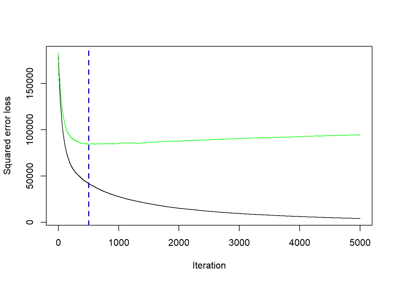
## var rel.inf
## Walks Walks 11.320578
## CRBI CRBI 10.877212
## CHmRun CHmRun 10.297120
## CRuns CRuns 8.237119
## CAtBat CAtBat 7.714124
## CWalks CWalks 7.677176
## RBI RBI 5.678778
## CHits CHits 5.651414
## Assists Assists 4.570534
## PutOuts PutOuts 4.353594
## HmRun HmRun 4.071464
## Runs Runs 3.955627
## Years Years 3.300331
## AtBat AtBat 2.982853
## Hits Hits 2.908079
## Division Division 2.395454
## Errors Errors 2.294263
## League League 1.714280
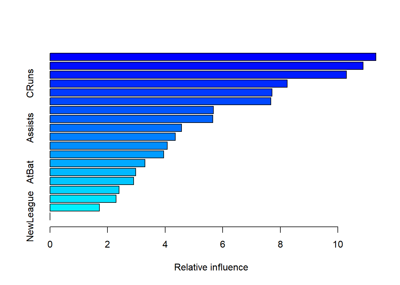
## NewLeague NewLeague 0.000000The summary() function produces a relative influence plot and also outputs the relative influence statistics.
boost_pred <- predict(boost_fit, newdata = Hitters_test, n.trees = Bhat)
mean((Hitters_test$Salary - boost_pred)^2)
## [1] 92857.11
In this particular dataset, random forest performs sligtly better than boosting (with this set of tuning parameters).