Chapter 2 Probability and Simulation

Optional Reading: R Cookbook Ch8

2.1 Probability Distributions

Using the normal distribution as an example:

Function	Purpose
dnorm	Normal density
pnorm	Normal CDF
qnorm	Normal quantile function
rnorm	Normal random variables

Examples

Density of $N(2, 3^2)$ at $5$.

dnorm(5, mean = 2, sd = 3)
## [1] 0.08065691

$P(X \leq 3)$, where $X \sim N(2, 3^2)$

pnorm(3, mean = 2, sd = 3)
## [1] 0.6305587
# "mean =" and "sd =" are optional
pnorm(3, 2, 3)
## [1] 0.6305587

Generate 10 random variables, each follows $N(3, 4^2)$.

rnorm(10, 3, 4)
##  [1]  3.0697823  5.7833862 -0.3445385  1.7289238
##  [5]  5.2347737 -2.6807430  2.6884267  4.2905353
##  [9]  3.2931281  2.9978411

95th percenttile of $N(0, 1)$. Find $q$ such that $P(Z \leq q) = 0.95$

qnorm(0.95, 0, 1)
## [1] 1.644854

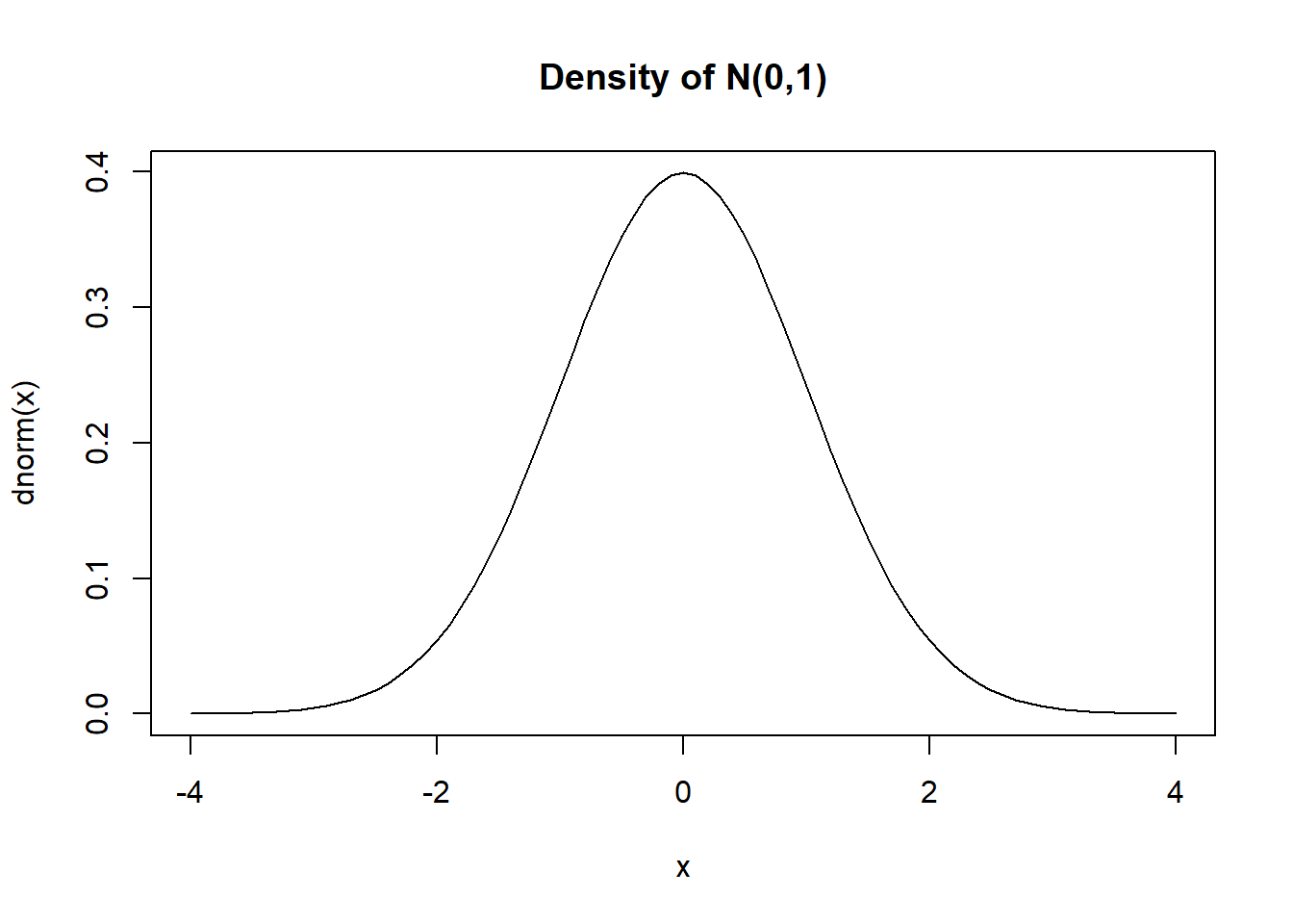
Plotting the normal density

x <- seq(-4, 4, by = 0.1)
plot(x, dnorm(x), type = "l", main = "Density of N(0,1)") # "l" for lines

2.1.1 Common Distributions

Common discrete distributions

Discrete distribution	R name	Parameters
Binomial	binom	n = number of trials; p = probability of success for one trial
Geometric	geom	p = probability of success for one trial
Negative binomial (NegBinomial)	nbinom	size = number of successful trials; either prob = probability of successful trial or mu = mean
Poisson	pois	lambda = mean

Common continuous distributions

Continuous distribution	R name	Parameters
Beta	beta	shape1; shape2
Cauchy	cauchy	location; scale
Chi-squared (Chisquare)	chisq	df = degrees of freedom
Exponential	exp	rate
F	f	df1 and df2 = degrees of freedom
Gamma	gamma	rate; either rate or scale
Log-normal (Lognormal)	lnorm	meanlog = mean on logarithmic scale; sdlog = standard deviation on logarithmic scale
Logistic	logis	location; scale
Normal	norm	mean; sd = standard deviation
Student’s t (TDist)	t	df = degrees of freedom
Uniform	unif	min = lower limit; max = upper limit

To get help on the distributions:

?dnorm
?dbeta
?dcauchy

# the following distributions need to use different code
?TDist
?Chisquare
?Lognormal

Examples (Using Binomial as an Example)

dbinom(2, 10, 0.6) # p_X(2), p_X is the pmf of X, X ~ Bin(n=10, p=0.6)
## [1] 0.01061683

pbinom(2, 10, 0.6) # F_X(2), F_X is the CDF of X, X ~ Bin(n=10, p=0.6)
## [1] 0.01229455

qbinom(0.5, 10, 0.6) # 50th percentile of X
## [1] 6

rbinom(4, 10, 0.6) # generate 4 random variables from Bin(n=10, p=0.6)
## [1] 8 4 9 5

x <- 0:10
plot(x, dbinom(x, 10, 0.6), type = "h") # "h" for histogram like vertical lines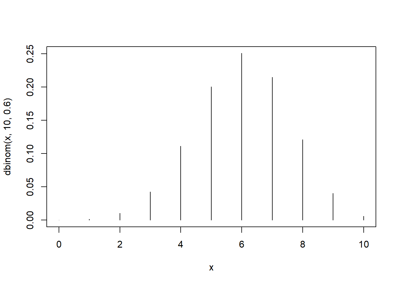

2.1.2 Exercises

1. The average number of trucks arriving on any one day at a truck depot in a certain city is known to be 12. Assuming the number of trucks arriving on any one day has a Poisson distribution, what is the probability that on a given day fewer than 9 (strictly less than 9) trucks will arrive at this depot?

ppois(8, 12)
## [1] 0.1550278

2. Let $Z \sim N(0, 1)$. Find $c$ such that

1. $P(Z \leq c) = 0.1151$

qnorm(0.1151)
## [1] -1.199844

2. $P(1\leq Z \leq c) = 0.1525$

c <- qnorm(pnorm(1) + 0.1525) # draw a graph

# test the answer
pnorm(c) - pnorm(1)
## [1] 0.1525

3. $P(-c \leq Z \leq c) = 0.8164$.

# P(0 <= Z <= c) = 0.8164/2
# P(Z <= c) = 0.8164/2 + 0.5
c <- qnorm(0.8164 / 2 + 0.5)

# test our answer
pnorm(c)- pnorm(-c)
## [1] 0.8164

1. Plot the density of a chi-squared distribution with degrees of freedom $4$, from $x=0$ to $x=10$.
2. Find the 95th percentile of this distribution.

# note that a chi-squared r.v. is nonnegative
x <- seq(0, 10, by = 0.1)
plot(x, dchisq(x, df = 4), type = "l")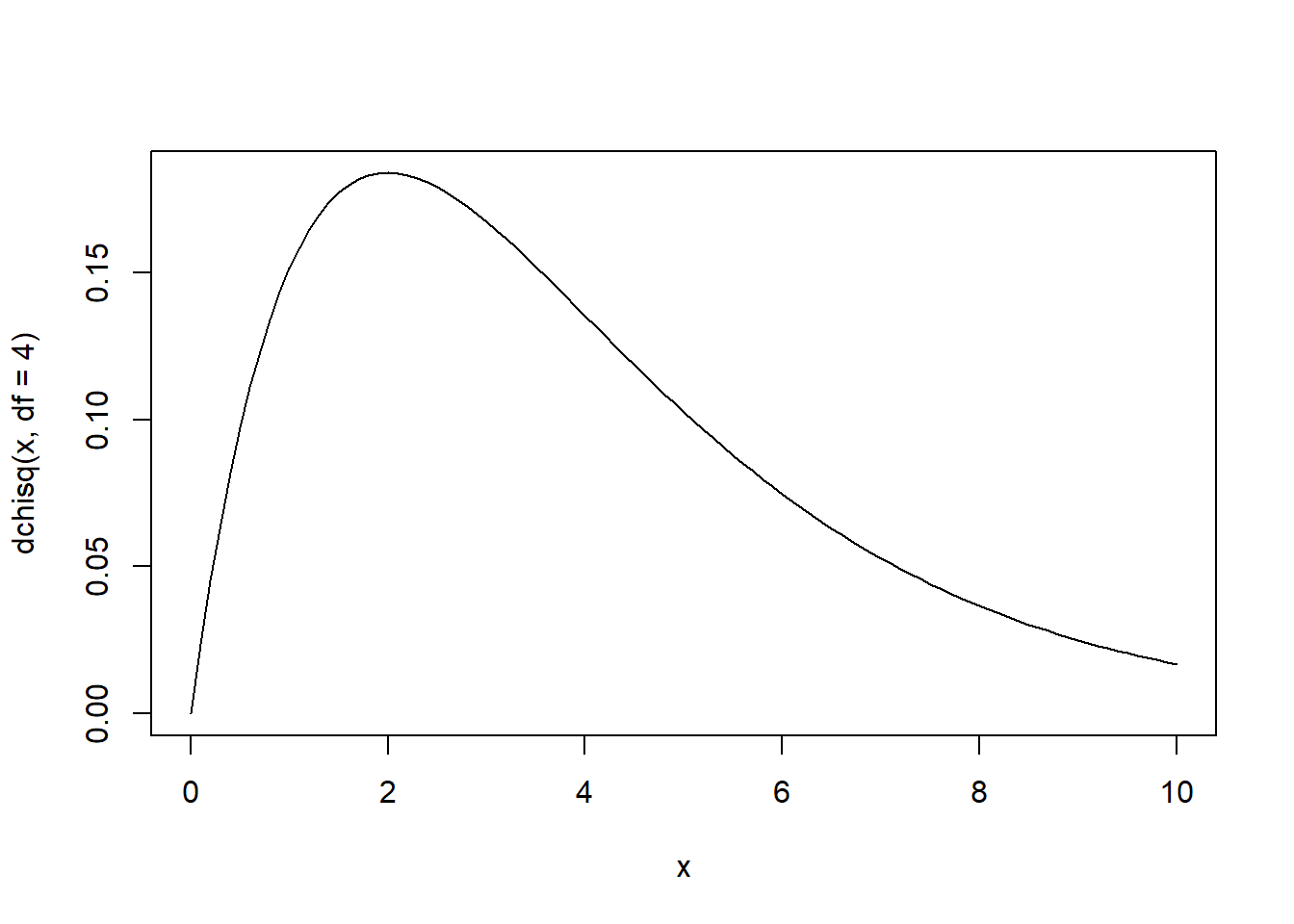

qchisq(0.95, df = 4)
## [1] 9.487729

4. Simulate $10$ Bernoulli random variables with parameter $0.6$.

# Bernoulli(p) = Bin(1, p)
rbinom(10, size = 1, prob = 0.6)
##  [1] 1 0 1 1 0 1 1 0 1 1

5. Plot the Poisson pmf with parameter $2$ from $x = 0$ to $x = 10$.

x <- 0:10
plot(x, dpois(x, 2), type = "h")

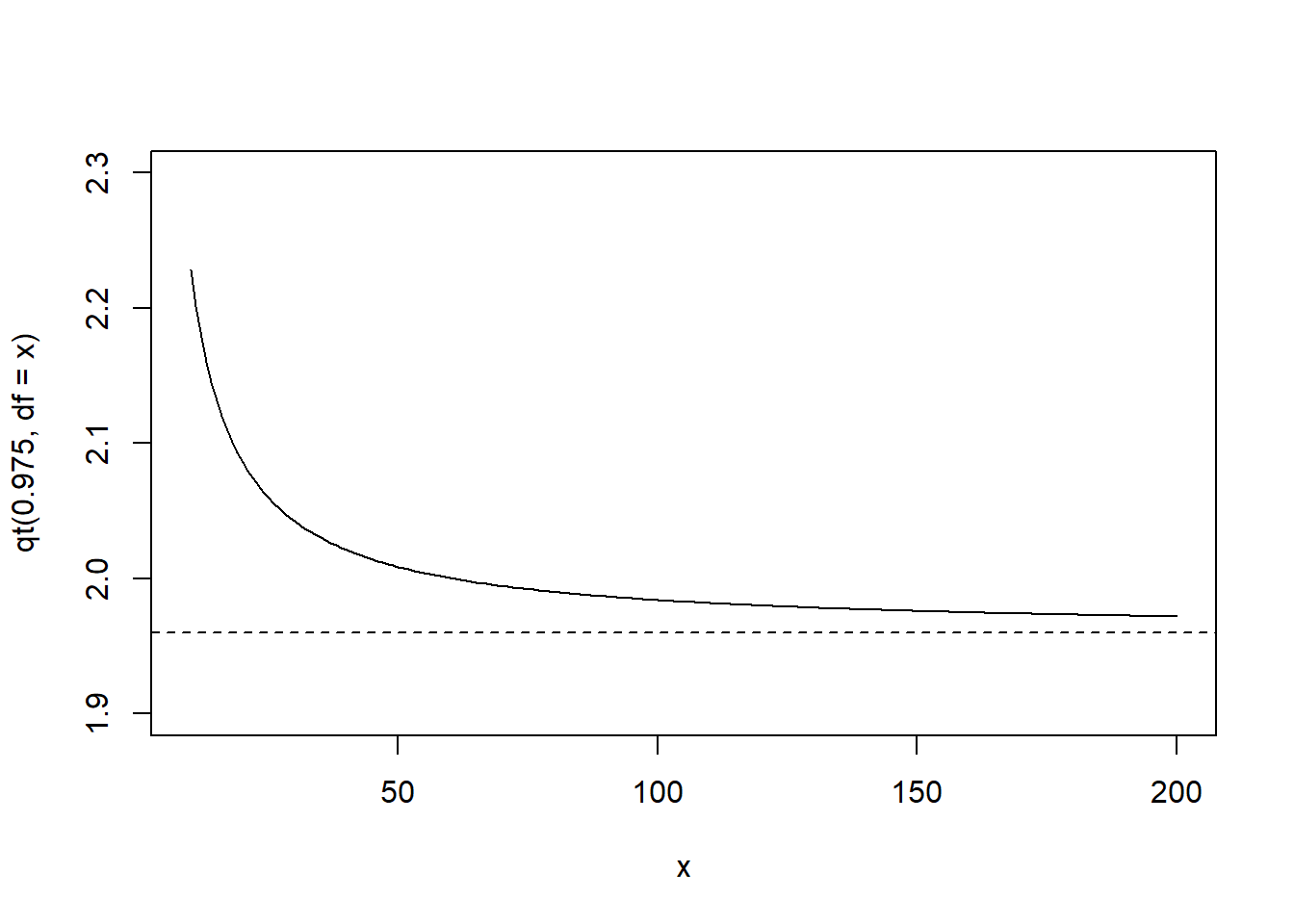
6. Draw a plot to illustrate that the 97.5th percentile of the t distribution will be getting closer to that of the standard normal distribution when the degrees of freedom increases.

x <- 10:200
plot(x, qt(0.975, df = x), type = "l", ylim = c(1.9,2.3))
# add a horizontal line with value at qnorm(0.975)
# lty = 2 for dashed line, check ?par
abline(h = qnorm(0.975), lty = 2) 

# Therefore, for a large sample, t-test and z-test will give you similar result.

2.2 Simulation

• We have already seen how to use functions like runif, rnorm, rbinom to generate random variables.

• R actually generates pseudo-random number sequence (deterministic sequence of numbers that approximates the properties of random numbers)

• The pseduo-random number sequence will be the same if it is initialized by the same seed (can be used to reproduce the same simulation results or used to debug).

# every time you run the first two lines, you get the same result
set.seed(1)
runif(5) 
## [1] 0.2655087 0.3721239 0.5728534 0.9082078 0.2016819

# every time you run the following code, you get a different result
runif(5)
## [1] 0.89838968 0.94467527 0.66079779 0.62911404
## [5] 0.06178627

Sampling from discrete distributions

Usage of sample:

sample(x, size, replace = FALSE, prob = NULL)

See also ?sample.

sample(10) # random permutation of integers from 1 to 10
##  [1]  3  1  5  8  2  6 10  9  4  7

sample(10, replace = T) # sample with replacement
##  [1]  5  9  9  5  5  2 10  9  1  4

sample(c(1, 3, 5), 5, replace = T) 
## [1] 5 3 3 3 3

# simulate 20 random variables from a discrete distribution
sample(c(-1,0,1), size = 20, prob = c(0.25, 0.5, 0.25), replace = T)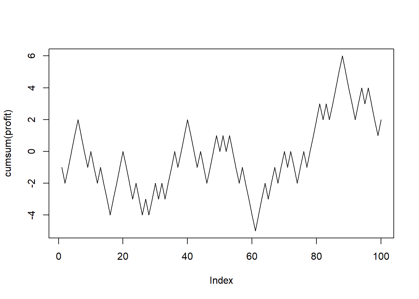
##  [1] -1  1  1 -1  0  0  1  1  0 -1  0  0  0  0  0  1
## [17]  1  0 -1  0

Example: Suppose we have a fair coin and we play a game. We flip the coin. We win $1 if the result is head and lose $1 if the result is tail. You play the game 100 times. You are interested in the cumulative profit.

set.seed(1) # R actually generates pseudo random numbers
# setting the seed ensure that each time you will get the same result
# for illustration, code debugging, reproducibility
profit <- sample(c(-1, 1), size = 100, replace = T)  
plot(cumsum(profit), type = "l")

set.seed(2) 
profit <- sample(c(-1, 1), size = 100, replace = T) 
plot(cumsum(profit), type = "l")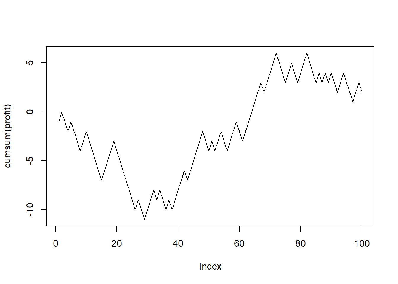

Example: You have two dice $A$ and $B$. For die $A$, there are $6$ sides with numbers $1,2,3,4,5,6$ and the corresponding probability of getting these values are $0.1,0.1,0.1,0.1,0.1,0.5$. For die $B$, there are $4$ sides with numbers $1,2,3,7$ and the corresponding probability of getting these values are $0.3,0.2,0.3,0.2$. You roll the two dice independently. Estimate $P(X > Y)$ using simulation, where $X$ is the result from die $A$ and $Y$ is the result from die $B$.

n <- 10000 # number of simulations
X <- sample(1:6, size = n, replace = TRUE, prob = c(0.1, 0.1, 0.1, 0.1, 0.1, 0.5))
Y <- sample(c(1, 2, 3, 7), size = n, replace = TRUE, prob = c(0.3, 0.2, 0.3, 0.2))
mean(X > Y)
## [1] 0.6408

Why the sample mean approximates the required probability? Recall the strong law of large numbers (SLLN). Let $X_1,\ldots,X_n$ be independent and identically distributed random variables with mean $\mu:=E(X)$. Let $\overline{X}_n:= \frac{1}{n} \sum^n_{i=1}X_i$. Then $$\overline{X}_n \stackrel{a.s.}{\rightarrow} \mu.$$ Note: a.s. means almost surely. The above convergence means $P(\lim_{n\rightarrow \infty} \overline{X}_n = \mu) = 1$. Note that (the expectation of an indicator random variable is the probability that the corresponding event will happen) $$P(X>Y) = E(I(X>Y)).$$ To apply SLLN, we just need to recognize the underlying random variable is $I(X>Y)$. Then, with probability $1$, the sample mean $$\frac{1}{n} \sum^n_{i=1} I(X_i > Y_i) \rightarrow P(X>Y).$$ The quantity on the LHS is what we compute in mean(X>Y) (note that we are using vectorized comparison).

2.3 Additional Exercises

Ex 1

Let $X \sim N(mean = 2, sd = 1)$, $Y \sim Exp(rate = 2)$, $Z \sim Unif(0, 4)$ (continuous uniform distribution on [0,4]). Suppose $X, Y, Z$ are independent. Estimate $P(\max(X,Y)>Z)$.

Recall the difference between pmax and max:

# always try with simple examples when you test the usage of functions
x <- c(1, 2, 3)
y <- c(0, 5, 10)
max(x, y)
## [1] 10
pmax(x, y)
## [1]  1  5 10

Answer:

n <- 100000
x <- rnorm(n, 2, 1)
y <- rexp(n, 2)
z <- runif(n, 0, 4)
mean(pmax(x, y) > z) 
## [1] 0.51129

Ex 2

Let $X \sim N(mean = 2, sd = 1)$, $Y \sim Exp(rate = 2)$, $Z \sim Unif(0, 4)$ (continuous uniform distribution on [0,4]). Suppose that $X, Y, Z$ are independent. Estimate $P(\min(X,Y)>Z)$.

n <- 100000
x <- rnorm(n, 2, 1)
y <- rexp(n, 2)
z <- runif(n, 0, 4)
mean(pmin(x, y) > z) # what is the difference between pmin and min?
## [1] 0.11283

Ex 3

Let $X \sim N(mean = 2, sd = 1)$, $Y \sim Exp(rate = 2)$, $Z \sim Unif(0, 4)$ (continuous uniform distribution on [0,4]). Suppose that $X, Y, Z$ are independent. Estimate $P(X^2 Y>Z)$.

n <- 100000
x <- rnorm(n, 2, 1)
y <- rexp(n, 2)
z <- runif(n, 0, 4)
mean(x ^ 2 * y > z)
## [1] 0.4084

Ex 4

Person $A$ generates a random variable $X \sim N(2, 1)$ and Person $B$ generates a random variable $Z \sim Unif(0, 4)$. If $X < Z$, Person $A$ will discard $X$ and generate another random variable $Y \sim Exp(0.5)$. Find the probability that the number generated by $A$ is greater than that by $B$.

n <- 100000
x <- rnorm(n, 2, 1)
y <- rexp(n, 0.5)
z <- runif(n, 0, 4)
mean(pmax(x, y) > z)
## [1] 0.63853

We will see additional simulation examples after we talk about some programming in R

There are many important topics that we will not discuss

1. algorithms for simulating random variables

• inverse transform
• acceptance rejection
• Markov Chain Monte Carlo

2. methods to reduce variance in simulation

• Control variates
• Antithetic variates
• Importance sampling