Chapter 7 Statistical Inference in R
In this chapter, we discuss how to perform parameter estimation and hypothesis testing in R. You may have learned the theoretical background in previous statistics courses. Here, the emphasis is on how these ideas are implemented in practice, rather than on a complete theoretical treatment. Because of time constraints, we focus on a few core ideas and representative examples.
Optional Readings:
- You can find a few more statistical tests in Ch 9 of R Cookbook (https://rc2e.com/)
- You can review Ch 10-13 of John E. Freund’s Mathematical Statistics with Applications by Irwin Miller and Marylees Miller (textbook for STAT 269) for some background and theory on statistical inference
7.1 Maximum Likelihood Estimation
After collecting data and specifying a statistical model, we need to estimate the unknown parameters. One of the most commonly used methods is maximum likelihood estimation (MLE).
Suppose we observe data \(y_1,\ldots,y_n\). The likelihood function is defined as \[\begin{equation*} L(\theta \mid y_1,\ldots,y_n) = f_{y_1,\ldots,y_n}(y_1,\ldots,y_n \mid \theta), \end{equation*}\] where \(f_{y_1,\ldots,y_n}(\cdot \mid \theta)\) is the joint pmf or pdf of the data given parameter \(\theta\).
If \(y_1,\ldots,y_n\) are independent and identically distributed with density \(f(\cdot \mid \theta)\), the likelihood simplifies to \[\begin{equation*} L(\theta \mid y_1,\ldots,y_n) = \prod_{i=1}^n f(y_i \mid \theta). \end{equation*}\]
The maximum likelihood estimator \(\hat\theta\) is the value of \(\theta\) that maximizes \(L(\theta \mid y_1,\ldots,y_n)\).
Some theory
Why maximize the likelihood?
- Intuition: the likelihood measures how plausible the observed data are under a given parameter value. Choosing the parameter that maximizes this quantity makes the observed data as likely as possible under the model.
- MLE has good statistical properties. Under some regularity conditions,
- MLE is consistent: \(\hat{\theta}_n\) converges in probability to \(\theta_0\)
- Asymptotically efficient: the estimator has the lowest variance asymptotically in some sense
- Asymptotically normality: can be used to find confidence intervals and perform hypothesis testings
Example (Logistic Regression): Suppose we observe \({(x_i, y_i) : i = 1,\ldots,n}\), where \(y_i \in {0,1}\) is a binary response and \(x_i\) is a vector of covariates (including an intercept).
In logistic regression, we assume \[\begin{equation*} P(Y_i = 1 \mid x_i, \beta) = \frac{e^{x_i^T \beta}}{1 + e^{x_i^T \beta}}. \end{equation*}\]
Equivalently, \[\begin{equation*} P(Y_i = y_i \mid x_i, \beta) = \frac{e^{(x_i^T \beta) y_i}}{1 + e^{x_i^T \beta}}, \qquad y_i \in {0,1}. \end{equation*}\]
The likelihood function (conditional on the covariates) is \[\begin{equation*} L(\beta \mid y, x) = \prod_{i=1}^n \frac{e^{(x_i^T \beta) y_i}}{1 + e^{x_i^T \beta}}. \end{equation*}\]
Taking logarithms gives the log-likelihood \[\begin{equation*} \sum_{i=1}^n \left[ (x_i^T \beta) y_i - \log(1 + e^{x_i^T \beta}) \right]. \end{equation*}\]
There is no closed-form solution for the maximizer, so numerical optimization is required.
Simulated Example and Why We Use Simulation
Before working with real data, it is often useful to simulate data from a known model. This allows us to answer two important questions:
- Is our estimation algorithm implemented correctly?
- Does the estimator behave as theory predicts when the model is correct?
In simulation, we know the true parameter values. If the estimation method is sensible, estimates should be close to the truth on average, and should improve as the sample size increases.
Step 1: Simulate data from a logistic regression model
set.seed(362)
n <- 1000
beta_0 <- c(0.5, 1, -1)

x1 <- runif(n, 0, 1)
x2 <- runif(n, 0, 1)

eta <- beta_0[1] + beta_0[2] * x1 + beta_0[3] * x2
prob <- exp(eta) / (1 + exp(eta))

y <- rbinom(n, size = 1, prob = prob)
Here, we first generate covariates \(x_1\) and \(x_2\), then compute the success probabilities using the logistic model, and finally generate binary responses.
Step 2: Define the negative log-likelihood
neg_log_like <- function(beta, y, x1, x2) {
  eta <- beta[1] + beta[2] * x1 + beta[3] * x2
  log_like <- sum(eta * y) - sum(log(1 + exp(eta)))
  -log_like
}
We minimize the negative log-likelihood because optim() performs minimization by default.
Step 3: Estimate the parameters using numerical optimization
optim(
  par = runif(3, 0, 1),
  f = neg_log_like,
  y = y, x1 = x1, x2 = x2,
  method = "BFGS"
)
## $par
## [1]  0.7830734  1.0067301 -1.4920231
##
## $value
## [1] 632.7284
##
## $counts
## function gradient
##       28        7
##
## $convergence
## [1] 0
##
## $message
## NULLparis the initial values for the optimization. We set some random numbers for the initial values bypar = runif(3, 0, 1).- Because the function
neg_log_likehave multiple arguments, we have to supply them insideoptim(). method = "BFGS"is a quasi-Newton method.method = "L-BFGS-B"is also useful when you want to add box constraints to your variable. You can check?optimto learn more about this.
Output:
paris the parameter values at which the minimum is obtainedvalueis the minimum function valueconvergence = 0indicates successful completion
Compare with the built-in function glm() for estimating the parameters:
# will discuss this in more detail later
fit <- glm(y ~ x1 + x2, family = "binomial")
fit
##
## Call:  glm(formula = y ~ x1 + x2, family = "binomial")
##
## Coefficients:
## (Intercept)           x1           x2
##      0.7831       1.0067      -1.4920
##
## Degrees of Freedom: 999 Total (i.e. Null);  997 Residual
## Null Deviance:       1324
## Residual Deviance: 1265  AIC: 1271
You can see that both methods give the same estimates 0.783, 1.007, -1.492 for the regression coefficients.
Using Simulation to Verify an Estimator
A single dataset is not enough to assess estimator performance. Even a good estimator can produce noisy results in one realization.
To better understand its behavior, we:
- Simulate many datasets from the same model
- Estimate the parameters for each dataset
- Examine the distribution of the estimates
Perform the simulation and estimation \(250\) times:
# Setting
n <- 1000
beta_0 <- c(0.5, 1, -1) # true beta
no_iter <- 250

beta_est <- matrix(0, nrow = no_iter, ncol = length(beta_0))

for (i in 1:no_iter) {
  # Simulation
  x1 <- runif(n)
  x2 <- runif(n)
  eta <- beta_0[1] + beta_0[2] * x1 + beta_0[3] * x2
  prob <- exp(eta) / (1 + exp(eta))
  y <- rbinom(n, 1, prob)

  # Estimation
  beta_est[i, ] <- optim(
    par = runif(3),
    f = neg_log_like,
    y = y, x1 = x1, x2 = x2,
    method = "BFGS"
  )$par
}
Visualizing the sampling distributions
library(tidyverse)

data <- tibble(
  est = c(beta_est[,1], beta_est[,2], beta_est[,3]),
  beta = rep(c("Beta1", "Beta2", "Beta3"), each = no_iter)
)

vline_data <- tibble(
  beta = c("Beta1", "Beta2", "Beta3"),
  mean = beta_0
)

ggplot(data, aes(x = est)) +
  geom_histogram(fill = "lightblue") +
  facet_grid(~ beta, scales = "free") +
  geom_vline(data = vline_data, aes(xintercept = mean), color = "blue")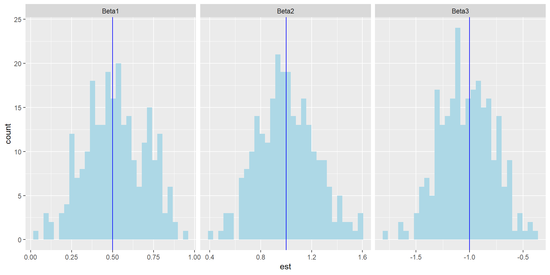
Observation:
Each histogram shows the sampling distribution of an estimator
The vertical line is the true parameter value
The distributions are centered near the truth, indicating approximate unbiasedness
Variability remains because the sample size is finite
Effect of increasing sample size
set.seed(362)
n <- 100000

x1 <- runif(n)
x2 <- runif(n)
eta <- beta_0[1] + beta_0[2] * x1 + beta_0[3] * x2
prob <- exp(eta) / (1 + exp(eta))
y <- rbinom(n, 1, prob)

optim(
  par = runif(3),
  f = neg_log_like,
  y = y, x1 = x1, x2 = x2,
  method = "BFGS"
)$par
## [1]  0.4803615  1.0275395 -0.9871783
With a larger sample size, the estimates are much closer to the true parameters. This illustrates consistency in practice.
We will see some applications of the logistic regression later.
7.1.1 Summary
MLE is a general and powerful estimation method
Numerical optimization is often required
Simulation helps verify correctness and understand estimator behavior
Repeated simulation reveals bias, variability, and consistency
Larger samples lead to more accurate estimation
7.1.2 Exercises on MLE
Exercise 1 (Gamma distribution)
You observe a random sample \(y_1,\ldots,y_n\) from a Gamma distribution with unknown parameters \(\alpha, \beta\). The likelihood function is \[\begin{equation*} L(\alpha, \beta |y_1,\ldots,y_n) = \prod^n_{i=1} \frac{\beta^\alpha}{\Gamma(\alpha)} y^{\alpha-1}_i e^{-\beta y_i}. \end{equation*}\] The log likelihood, after simpliciation, is \[\begin{equation*} \log L(\alpha, \beta) = n \alpha \log \beta - n \log \Gamma(\alpha) + (\alpha - 1) \sum^n_{i=1} \log y_i - \beta \sum^n_{i=1} y_i. \end{equation*}\]
# Setting
set.seed(1)
alpha <- 1.5
beta <- 2
n <- 10000

# Simulation
x <- rgamma(n, alpha ,beta)

# Optimization (Estimation)
Exercise 2 (Poisson Regression)
Suppose we observe \(\{(x_i, y_i):i=1,\ldots,n\}\), where \(y_i\) only takes nonnegative integer values (count data) and \(x_i\) is a vector of covariates (including the intercept \(1\)). In Poisson regression, we assume that \(Y_i\) has a Poisson distribution and \[\begin{equation*} \log (E(Y_i|x_i)) = \beta^T x_i = \beta_0 + \beta_1 x_{i1} + \ldots + \beta_p x_{ip}, \end{equation*}\] where \(\beta \in \mathbb{R}^{p+1}\). Alternatively, condition on \(x_i\), \(Y_i|x_i \sim \text{Pois}(e^{\beta^T x_i})\). The likelihood is \[\begin{equation*} L(\beta|y,x) = \prod^n_{i=1} \frac{e^{-e^{\beta^T x_i}} e^{(\beta^T x_i)y_i}}{y_i!}. \end{equation*}\] The log likelihood is \[\begin{equation*} \log L(\beta|y, x) = \sum^n_{i=1} \bigg( -e^{\beta^T x_i} + (\beta^T x_i) y_i - \log (y_i!) \bigg). \end{equation*}\] Clearly, the term \(\log (y_i !)\) does not depend on \(\beta\) and hence we do not need to consider it during our optimization. Therefore, it suffices to maximize (or minimize the negative of) the following objective function \[\begin{equation*} \sum^n_{i=1} \bigg( -e^{\beta^T x_i} + (\beta^T x_i) y_i \bigg). \end{equation*}\]
7.2 Interval Estimation and Hypothesis Testing
There are two main types of estimation:
Point estimation, which produces a single value (for example, the MLE).
Interval estimation, which produces a range of plausible values (for example, a confidence interval).
Hypothesis testing is closely related to interval estimation. Both aim to quantify uncertainty and help us decide whether the data are consistent with a proposed model or parameter value.
7.2.1 Examples of Hypothesis Testing
Optional reading: Chapter 12 in John E. Freund’s Mathematical Statistics with Applications.
Suppose you have a die and you wonder whether it is unbiased. If the die is unbiased, the (population) mean of one roll is \(3.5\).
If you roll the die \(10\) times and the sample mean is \(5\), what should you conclude?
How confident are you in that conclusion?
If you roll the die \(100\) times and the sample mean is still \(5\), would your conclusion change? Would you be more confident?
If you roll the die \(10\) times but the sample mean is \(4\), what would you conclude then?
To answer questions like these, we need tools for interval estimation and hypothesis testing.
More examples:
An engineer has to decide on the basis of sample data whether the true average lifetime of a certain kind of tire is at least \(42,000\) miles
An agronomist has to decide on the basis of experiments whether one kind of fertilizer produces a higher yield of soybeans than another
A manufacturer of pharmaceutical products has to decide on the basis of samples whether 90 percent of all patients given a new medication will recover from a certain disease
These can all be expressed using the language of statistical tests of hypotheses:
the engineer has to test the hypothesis that \(\theta\), the parameter of an exponential population, is at least \(42,000\)
the agronomist has to decide whether \(\mu_1 > \mu_2\), where \(\mu_1\) and \(\mu_2\) are the means of two normal populations
the manufacturer has to decide whether \(\theta\), the parameter of a binomial population, equals \(0.90\)
In each case, we assume that the chosen distribution provides a reasonable statistical model for the data-generating process.
7.2.2 Null Hypotheses, Alternative Hypotheses, and p-values
An assertion or conjecture about the distribution of one or more random variables is called a statistical hypothesis.
If a statistical hypothesis completely specifies the distribution, it is called a simple hypothesis; if not, it is referred to as a composite hypothesis.
Null hypothesis (\(H_0\)): the hypothesis we treat as the default position and test against. Historically, \(H_0\) often represented “no difference,” but in modern usage it can be any hypothesis of interest.
Alternative hypothesis (\(H_1\)): what we consider plausible if the data are not consistent with \(H_0\).
p-value: the probability, assuming \(H_0\) is true, of obtaining a test statistic at least as extreme as the one observed.
Steps in Hypothesis Testing
- Assume \(H_0\) is true.
- Compute a test statistic (for example, a sample mean).
- Compute a p-value using the sampling distribution of the statistic under \(H_0\).
For example, if the die is unbiased, what is the probability that the sample mean exceeds \(5\) after rolling it \(100\) times?
- small \(p\)-value: the observed statistic would be unlikely if \(H_0\) were true, so we have evidence against \(H_0\).
- large \(p\)-value: the observed statistic is not unusual under \(H_0\), so we do not have enough evidence to reject \(H_0\).
Remark
In this course, we will follow the common convention of rejecting \(H_0\) when \(p < 0.05\).
In real applications, what counts as “small” depends on the context and consequences of errors.
Statistical significance (small p-value) does not imply that the difference is practically important. It is often helpful to also examine confidence intervals or the magnitude of the estimated effect.
7.2.3 Type I error and Type II error
Type I error: rejecting \(H_0\) when \(H_0\) is true. The probability of a Type I error is denoted by \(\alpha\) (the significance level).
Type II error: failing to reject \(H_0\) when \(H_0\) is false. The probability of a Type II error is denoted by \(\beta\).
| \(H_0\) is true | \(H_1\) is true | |
|---|---|---|
| Reject \(H_0\) | Type I error | No Error |
| Do not reject \(H_0\) | No Error | Type II Error |
A good testing procedure keeps both \(\alpha\) and \(\beta\) small. However, for a fixed sample size \(n\), decreasing \(\alpha\) typically increases \(\beta\), and vice versa. Increasing the sample size is the main way to reduce both types of error probabilities.
In practice, we usually choose a small value of \(\alpha\), such as \(0.05\), and then evaluate power (which is \(1-\beta\)) under meaningful alternatives.
7.2.4 Inference for Mean of One Sample
Hypothesis Testing Problem
You have a random sample \(X_1,\ldots,X_n\) from a population. You want to test whether the population mean \(\mu\) equals a specified value \(\mu_0\): \[\begin{equation*} H_0: \mu =\mu_0 \quad vs. \quad H_1:\mu \neq \mu_0 \end{equation*}\]
Solution
You can use the \(t\)-test for this problem. It is appropriate when either
- Your data is normally distributed
- You have a large sample size \(n\). A rule of thumb is \(n > 30\).
The test statistic is
\[\begin{equation*}
\frac{\overline{X}_n - \mu_0}{s/\sqrt{n}},
\end{equation*}\]
where \(\overline{X}_n\) is the sample mean and \(s\) is the sample standard deviation. In R, use t.test() to perform the t-test.
# Simulate the data
set.seed(362) # so that you can replicate the result
x <- rnorm(75, mean = 100, sd = 15)

# Perform t-test
t.test(x, mu = 95)
##
##  One Sample t-test
##
## data:  x
## t = 4.7246, df = 74, p-value = 1.071e-05
## alternative hypothesis: true mean is not equal to 95
## 95 percent confidence interval:
##   99.36832 105.74018
## sample estimates:
## mean of x
##  102.5543
The p-value is small, which indicates that a population mean of \(95\) would be unlikely given this sample.
[Optional] How are the test statistic and \(p\)-value calculated?
The \(p\)-value in this case is \(2 \times P_{H_0}(T > |\text{obs. T.S.|})\), where \(T\) has a \(t\)-distribution with degrees of freedom \(n-1\) if the data from are from a normal distribution and obs. T.S. stands for the observed test statistic. The subscript \(H_0\) is to stress that the probability measure is under \(H_0\).
# test statistic
(obs_ts <- (mean(x) - 95) / (sd(x) / sqrt(length(x))))
## [1] 4.724574

# p-value
2 * (1 - pt(abs(obs_ts), df = length(x) - 1))
## [1] 1.071253e-05
What happens if the population variance is much larger?
set.seed(362) # so that you can replicate the result
x2 <- rnorm(75, mean = 100, sd = 200)
(test_x2 <- t.test(x2, mu = 95))
##
##  One Sample t-test
##
## data:  x2
## t = 1.832, df = 74, p-value = 0.07097
## alternative hypothesis: true mean is not equal to 95
## 95 percent confidence interval:
##   91.57758 176.53580
## sample estimates:
## mean of x
##  134.0567
Even if the estimate of the population mean is 134, the test does not reject \(H_0\) because the data are highly variable. Large variability makes it harder to detect differences in the mean.
Interval Estimation
Let \(\overline{x}n\) and \(s_n\) be the sample mean and sample standard deviation. A \(100(1-\alpha)%\) confidence interval for \(\mu\) is \[\begin{equation*} \bigg[ \overline{x}_n - t_{n-1;\alpha/2} \frac{s_n}{\sqrt{n}}, \overline{x}_n + t_{n-1;\alpha/2} \frac{s_n}{\sqrt{n}} \bigg], \end{equation*}\] where \(t_{n-1;\alpha/2}\) satisfies \(P(T > t_{n-1;\alpha/2})=\alpha/2\) and \(T \sim t(n-1)\).
In R, use t.test() to get a confidence interval. For example, a \(99%\) confidence interval:
t.test(x, conf.level = 0.99)
##
##  One Sample t-test
##
## data:  x
## t = 64.139, df = 74, p-value < 2.2e-16
## alternative hypothesis: true mean is not equal to 0
## 99 percent confidence interval:
##   98.32683 106.78168
## sample estimates:
## mean of x
##  102.5543
Remark
- If you omit
mu = ...,t.test()uses the default null valuemu = 0. If your goal is only the confidence interval, the choice ofmuis irrelevant.
[Optional] Computing the confidence interval without t.test():
alpha <- 0.01
n <- length(x)
half_width <- qt(1 - alpha / 2, n - 1) * sd(x) / sqrt(n)

c(mean(x) - half_width, mean(x) + half_width)
## [1]  98.32683 106.78168
Interpretation
If you repeat the sampling procedure many times and compute a \(95\%\) confidence interval each time, then about \(95\%\) of those intervals will contain the true mean.
no_sim <- 10000
set.seed(362) # so that you can replicate the result
true_mean <- 100
CI <- matrix(0, nrow = no_sim, ncol = 2)

for (i in 1:no_sim) {
  CI[i, ] <- t.test(rnorm(75, mean = true_mean, sd = 200))$conf.int
}

# find out the proportion of CIs that contain 0
mean(CI[, 1] < 100 & 100 < CI[, 2])
## [1] 0.9503
Example: Confidence Interval for a Simulation Estimate
Recall that we can estimate \(P(X > Y)\) by simulation. For example, let \(X \sim N(0,1)\), \(Y \sim \mathrm{Exp}(2)\), independent. Then \(I(X>Y)\) is a Bernoulli random variable with mean \(P(X>Y)\), so the simulation estimate is a sample proportion.
We can attach a confidence interval to this Monte Carlo estimate using t.test():
t.test(X > Y)
##
##  One Sample t-test
##
## data:  X > Y
## t = 70.162, df = 9999, p-value < 2.2e-16
## alternative hypothesis: true mean is not equal to 0
## 95 percent confidence interval:
##  0.3206831 0.3391169
## sample estimates:
## mean of x
##    0.3299
We see that the \(95\%\) CI is (0.321, 0.339). If we increase the number of simulations, the confidence interval becomes narrower:
set.seed(1)
n <- 1000000
X <- rnorm(n, 0, 1)
Y <- rexp(n, 2)

t.test(X > Y)
##
##  One Sample t-test
##
## data:  X > Y
## t = 704.63, df = 1e+06, p-value < 2.2e-16
## alternative hypothesis: true mean is not equal to 0
## 95 percent confidence interval:
##  0.3308521 0.3326979
## sample estimates:
## mean of x
##  0.331775
The \(95\%\) CI becomes (0.331, 0.333).
The width of the confidence interval scales roughly like \(1/\sqrt{n}\): \[\begin{equation*} 2 \times t_{n-1;\alpha/2}\frac{s}{\sqrt{n}}. \end{equation*}\] This relationship can be used to determine how many simulation runs are needed to achieve a desired level of accuracy.
7.2.5 Comparing the means of two samples
Suppose you have two samples from two populations and want to test whether the population means are equal.
\[\begin{equation*} H_0: \mu_1 = \mu_2 \text{ and } H_1: \mu_1 \neq \mu_2. \end{equation*}\]
There are two common \(t\)-tests (assuming normality or large samples):
the observations are not paired
the observations are paired
To clarify paired data, consider two experiments testing whether morning coffee improves test scores:
Unpaired observations: two independent groups, one drinks coffee and one does not. Each person contributes one score.
Paired observations: the same individuals take the test twice, once with coffee and once without. Each person contributes two scores, which are dependent.
Example
We illustrate the paired \(t\)-test using the dataset sleep (no package is required). The data contains the increase in hours of sleep when the subject took two soporific drugs compared to control on \(10\) subjects. Since each subject received two drugs, the observations are paired.
Take a look at sleep:
sleep
##    extra group ID
## 1    0.7     1  1
## 2   -1.6     1  2
## 3   -0.2     1  3
## 4   -1.2     1  4
## 5   -0.1     1  5
## 6    3.4     1  6
## 7    3.7     1  7
## 8    0.8     1  8
## 9    0.0     1  9
## 10   2.0     1 10
## 11   1.9     2  1
## 12   0.8     2  2
## 13   1.1     2  3
## 14   0.1     2  4
## 15  -0.1     2  5
## 16   4.4     2  6
## 17   5.5     2  7
## 18   1.6     2  8
## 19   4.6     2  9
## 20   3.4     2 10
The sleep data is in a long format. Let’s turn it into a wide format using spread, a function in the package tidyr, which is contained in tidyverse.
(sleep_wide <- spread(sleep, group, extra))
##    ID    1    2
## 1   1  0.7  1.9
## 2   2 -1.6  0.8
## 3   3 -0.2  1.1
## 4   4 -1.2  0.1
## 5   5 -0.1 -0.1
## 6   6  3.4  4.4
## 7   7  3.7  5.5
## 8   8  0.8  1.6
## 9   9  0.0  4.6
## 10 10  2.0  3.4
Paired \(t\)-test:
t.test(sleep_wide[, 2], sleep_wide[, 3], paired = TRUE)
##
##  Paired t-test
##
## data:  sleep_wide[, 2] and sleep_wide[, 3]
## t = -4.0621, df = 9, p-value = 0.002833
## alternative hypothesis: true mean difference is not equal to 0
## 95 percent confidence interval:
##  -2.4598858 -0.7001142
## sample estimates:
## mean difference
##           -1.58
The \(p\)-value is \(< 0.05\). We conclude that the effect of the two drugs are different. The \(95\%\) CI of the difference between the two means is (-2.46, -0.70).
Example
Are the means of the birth weights in the smoking group and non-smoking group different?
library(MASS)
t.test(birthwt$bwt[birthwt$smoke == 1], birthwt$bwt[birthwt$smoke == 0])
##
##  Welch Two Sample t-test
##
## data:  birthwt$bwt[birthwt$smoke == 1] and birthwt$bwt[birthwt$smoke == 0]
## t = -2.7299, df = 170.1, p-value = 0.007003
## alternative hypothesis: true difference in means is not equal to 0
## 95 percent confidence interval:
##  -488.97860  -78.57486
## sample estimates:
## mean of x mean of y
##  2771.919  3055.696
The \(p\)-value is \(< 0.05\). We conclude that the means are different. The \(95\%\) CI of the difference between the two means is (-489.0, -78.6).
7.2.6 Inference of a Sample Proportion
You observe independent successes and failures from a population. You want to test whether the true success probability \(p\) equals a given value \(p_0\). \[\begin{equation*} H_0: p = p_0 \text{ and } H_1: p \neq p_0 \end{equation*}\]
Example: testing coin fairness
You flip a coin \(100\) times independently. You want to test if the coin is fair \((p_0 = 0.5)\).
# Simulate the coin flips
set.seed(1)
heads <- rbinom(1, size = 100, prob = .4)

# Test, p_0 = 0.5
(result <- prop.test(heads, 100, p = 0.5))
##
##  1-sample proportions test with continuity correction
##
## data:  heads out of 100, null probability 0.5
## X-squared = 2.25, df = 1, p-value = 0.1336
## alternative hypothesis: true p is not equal to 0.5
## 95 percent confidence interval:
##  0.3233236 0.5228954
## sample estimates:
##    p
## 0.42
The point estimate is 0.42. Although the true probability of success used in the simulation is \(0.4\), for this particular data, we do not reject to null hypothesis that the true probability of success is \(0.5\) as the \(p\)-value equals 0.134, which is larger than \(0.05\). The 95% confidence interval is equal to (0.323, 0.523).
One-sided alternatives are also possible (\(p > p_0\) or \(p < p_0\)):
prop.test(heads, 100, p = 0.5, alternative = "greater")
##
##  1-sample proportions test with continuity correction
##
## data:  heads out of 100, null probability 0.5
## X-squared = 2.25, df = 1, p-value = 0.9332
## alternative hypothesis: true p is greater than 0.5
## 95 percent confidence interval:
##  0.3372368 1.0000000
## sample estimates:
##    p
## 0.42

prop.test(heads, 100, p = 0.5, alternative = "less")
##
##  1-sample proportions test with continuity correction
##
## data:  heads out of 100, null probability 0.5
## X-squared = 2.25, df = 1, p-value = 0.06681
## alternative hypothesis: true p is less than 0.5
## 95 percent confidence interval:
##  0.0000000 0.5072341
## sample estimates:
##    p
## 0.42
7.2.7 Testing groups for equal proportions
You have binary outcomes from two or more groups and want to test whether all groups share the same success probability.
Example
# 3 groups
no_success <- c(48, 60, 50) # no. of successes in the 3 groups
no_trial <- c(100, 100, 100) # corresponding no. of trails in the 3 groups
prop.test(no_success, no_trial)
##
##  3-sample test for equality of proportions without continuity correction
##
## data:  no_success out of no_trial
## X-squared = 3.3161, df = 2, p-value = 0.1905
## alternative hypothesis: two.sided
## sample estimates:
## prop 1 prop 2 prop 3
## 0.48 0.60 0.50\(p\)-value is \(> 0.05\). We do not reject the null hypothesis that the three groups have the same proportion of success.
Example
In a class of \(38\) students, \(14\) of them got \(A\). In another class of \(40\) students, only \(10\) got \(A\). We want to know if the difference between the two proportions is statistically significant.
prop.test(c(14, 10), c(38, 40))
##
##  2-sample test for equality of proportions with continuity correction
##
## data:  c(14, 10) out of c(38, 40)
## X-squared = 0.7872, df = 1, p-value = 0.3749
## alternative hypothesis: two.sided
## 95 percent confidence interval:
##  -0.1110245  0.3478666
## sample estimates:
##    prop 1    prop 2
## 0.3684211 0.2500000
The \(p\)-value is \(> 0.05\). We do not reject the null hypothesis that the students in the two groups have the same proportion of getting an A.
7.2.8 Testing if two samples have the same underlying distribution
Problem
You have two random samples \(X_1,\ldots,X_n\) and \(Y_1,\ldots,Y_m\). Let \(F\) and \(G\) be the distribution functions of \(X_i\)’s and \(Y_i\)’s respectively. You want to know if \(F \equiv G\).
\[\begin{equation*} H_0: F = G \text{ and } H_1: F \neq G. \end{equation*}\]
Solution
You may use the Kolmogorov-Smirnov test.
- It does not require any assumptions.
- The test statistic is \[ D := \sup_{x \in \mathbb{R}}|F_n(x) - G_m(x)|,\] where \(F_n\) and \(G_m\) are the empirical distribution functions of \(X_i\)’s and \(Y_i\)’s respectively. That is, \[ F_n(x) := \frac{1}{n} \sum^n_{i=1} I(X_i \leq x)\] and \[ G_m(x) := \frac{1}{m} \sum^m_{i=1} I(Y_i \leq x).\]
Example
set.seed(362)
x <- rnorm(100, 0, 1)
y <- rnorm(100, 0, 1)
ks.test(x, y)
##
##  Asymptotic two-sample Kolmogorov-Smirnov test
##
## data:  x and y
## D = 0.07, p-value = 0.9671
## alternative hypothesis: two-sided
The \(p\)-value is not small. We do not have enough evidence to reject the null hypothesis that the two distributions are the same.
Example
z <- rnorm(100, 2, 1)
ks.test(y, z)
##
##  Asymptotic two-sample Kolmogorov-Smirnov test
##
## data:  y and z
## D = 0.77, p-value < 2.2e-16
## alternative hypothesis: two-sided
The \(p\)-value is very small. We will reject the null hypothesis that the two distributions are the same.
Example with birthwt
Recall the dataset birthwt from the package MASS. We created the following histograms to visualize the distributions of birth weights for the two groups (smoke and no smoke).
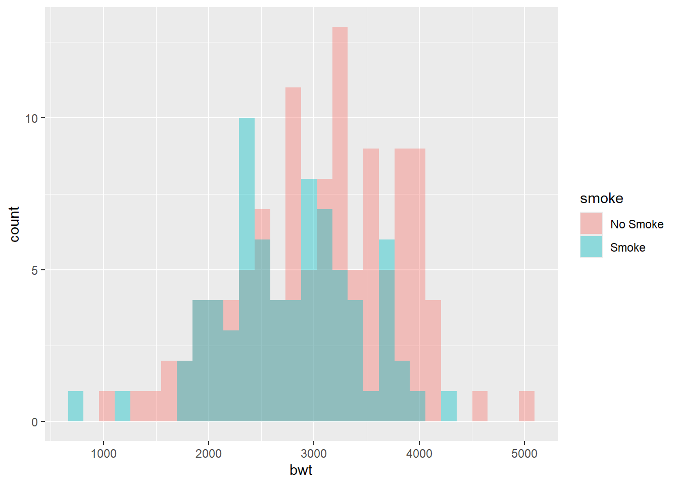
We may want to ask if the two distributions are different
ks.test(birthwt$bwt[birthwt$smoke == 0], birthwt$bwt[birthwt$smoke == 1])
##
##  Exact two-sample Kolmogorov-Smirnov test
##
## data:  birthwt$bwt[birthwt$smoke == 0] and birthwt$bwt[birthwt$smoke == 1]
## D = 0.21962, p-value = 0.01915
## alternative hypothesis: two-sided
The \(p\)-value is smaller than \(0.05\). Therefore, we conclude that the difference of the two distributions is statistically significant.