Chapter 8 Root finding and optimization
Reference: Computational Methods for Numerical Analysis with R by James P. Howard, II
Packages used:
In this chapter, some basic algorithms for root finding and optimization are introduced. A root of a function means the \(x\) such that \(f(x) = 0\). We will also discuss how to implement them in R to practise your code writing ability.
8.1 Root Finding
8.1.1 Bisection Method
Game: Before we introduce the bisection method, consider a game where Player \(A\) picks an integer from \(1\) to \(100\), and Player \(B\) has to guess this number. Player \(A\) will tell Player \(B\) if the guess is too low or too high. For example,
- Player \(A\) picks \(10\).
- Player \(B\) guesses \(40\).
- Player \(A\) tells Player \(B\) the number is too high.
- Player \(B\) will then pick a number from \(1\) to \(40\), say, \(28\).
- Play \(A\) tells Player \(B\) the number is also too high.
Eventually, Player \(B\) can guess the number correctly. You may realize that the best approach is to halve the range with each turn.
Idea of Bisection Method:
Recall that for any continuous function \(f\), if it has values of opposite sign in an interval, then it has a root in the interval. For example, if \(f(a) < 0\) and \(f(b) > 0\), then there exists \(c \in (a, b)\) such that \(f(c) = 0\).
Now, suppose that \(f(a) f(b) < 0\) (so that \(f\) has values of opposite sign at \(a\) and \(b\)). Let \(\varepsilon\) denote a tolerance level.
Algorithm:
- Let \(c = \frac{a + b}{2}\).
- If \(f(c) = 0\), stop and return \(c\).
- If \(\text{sign}(f(a)) \neq \text{sign}(f(c))\); set \(b = c\); else set \(a = c\).
- Repeat Step 1 to 3 until \(|b-a| < \varepsilon\).
Implementation in R:
This is a good example to see when a while loop is useful.
bisection <- function(f, a, b, tol = 1e-5, max_iter = 100) {
  iter <- 0

  # Step 4
  while (abs(b - a) > tol) {
    # Step 1
    c <- (a + b) / 2

    # Step 2: if f(c) = 0, stop and return c
     if (f(c) == 0) {
      return(c)
    }

    iter <- iter + 1
    if (iter > max_iter) {
      warning("Maximum number of iterations reached")
      return(c)
    }

    # Step 3
    if (f(a) * f(c) < 0) {
      b <- c
    } else {
      a <- c
    }
    # print(round(c(c, f(c)), digits = 3))
  }
  return((a + b) / 2)
}
Remark: 1e-3 = 0.001. We set the default value of \(\varepsilon\) to \(0.001\) and the maximum number of iterations to \(100\).
Example
Without providing the values of tol and max_iter, the function will use tol = 1e-3 and max_iter = 100.
To change tol:
bisection(f, 0.5, 1.25, tol = 0.1)
## [1] 1.015625

bisection(f, 0.5, 1.25, tol = 0.0000001)
## [1] 1
To change max_iter:
8.2 Newton-Raphson Method
Newton-Raphson method can be used to find a root of a function.
Idea of Netwon-Raphson Method (or Netwon’s Method):
Given an initial estimate of the root \(x_0\), approximate your function by its tangent line at \(x_0\) and find the root (you can find the root of a line easily). To find the root, we equate the slope at \(x_0\) found by \(f'(x_0)\) and using the two points \((x_1, 0)\) and \((x_0, f(x_0))\), where \(x_1\) denotes the root of the tangent line at \(x_0\). That is, \[\begin{equation*} \frac{f(x_0) - 0}{x_0 - x_1} = f'(x_0). \end{equation*}\] Rearranging the terms give \[\begin{equation*} x_1 = x_0 - \frac{f(x_0)}{f'(x_0)}. \end{equation*}\]
Iterate the above procedure until convergence.
Here is an gif animination from wikipedia: https://en.wikipedia.org/wiki/Newton%27s_method#/media/File:NewtonIteration_Ani.gif
Algorithm of Netwon-Raphson Method:
Given an initial estimate of the root \(x_0\), set \[\begin{equation*} x_1 = x_0 - \frac{f(x_0)}{f'(x_0)}. \end{equation*}\]
Iterate the following equation until convergence \[\begin{equation*} x_n = x_{n-1} - \frac{f(x_{n-1})}{f'(x_{n-1})}. \end{equation*}\]
Implementation in R:
fis the function you want to find the rootfpis the first derivative offx0is the initial value.- Since we cannot iterate indefinitely, we have to set a tolerance (
tol) and a maximum number of iteration (max_iter).
NR <- function(f, fp, x0, tol = 1e-3, max_iter = 100) {
  iter <- 0
  old_x <- x0
  x <- old_x + 10 * tol # any number such that abs(x - old_x) > tol

  while(abs(x - old_x) > tol) {
    iter <- iter + 1
    if (iter > max_iter) {
      print("Maximum number of iterations reached")
      return(x)
    }
    old_x <- x
    x <- x - f(x) / fp(x)
  }
  return(x)
}
Symbolic differentiation
To perform symbolic differentiation in R (instead of numerical differentiation), we can use Deriv() in the package Deriv.
f <- function(x) {
  x^2 - 2 * x + 1
}

# Symbolic differentiation
fp <- Deriv(f)

fp # we know it is 2x - 2
## function (x)
## 2 * x - 2
Apply our NR function
Let’s plot the function first.
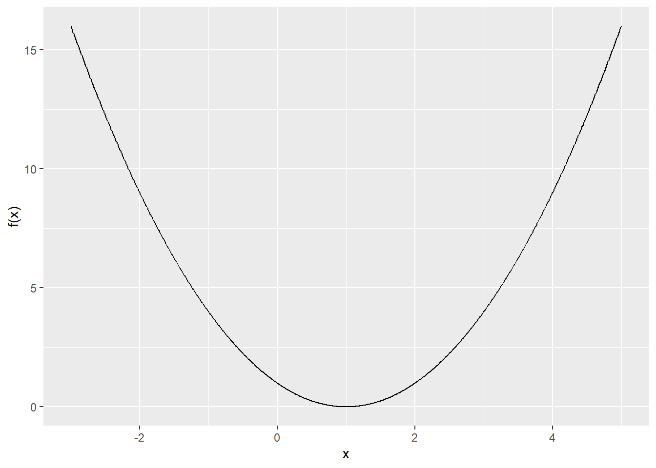
Using our function:
8.3 Minimization and Maximization
8.3.1 Newton-Raphson Method
Recall that at local extrema, \(f'(x) = 0\), therefore we can use the Netwon-Raphson method for minimization and maximization.
Algorithm of Netwon-Raphson Method:
Given an initial estimate of the root \(x_0\), set \[\begin{equation*} x_1 = x_0 - \frac{f'(x_0)}{f''(x_0)}. \end{equation*}\]
Iterate the following equation until convergence \[\begin{equation*} x_n = x_{n-1} - \frac{f'(x_{n-1})}{f''(x_{n-1})}. \end{equation*}\]
Multivariate Version
Iterate the following equation until convergence: \[\begin{equation*} x_n = x_{n-1} - [f''(x_{n-1})]^{-1} f'(x_{n-1}), \end{equation*}\] where \(f'(x)\) is the gradient and \(f''(x)\) is the Hessian matrix.
Example (Logistic Regression)
Recall that \(x_i = (x_{i1},\ldots,x_{ip})^T\) and \(y = (y_1,\ldots,y_n)^T\).
Log-likelihood of the logistic regresison model:
\[\begin{equation*} l(\beta) = \sum^n_{i=1} \{(x^T_i \beta)y_i - \log (1 + e^{x^T_i \beta}) \}. \end{equation*}\]
To apply the Netwon’s method, we have to find the gradient and the Hessian matrix.
The gradient is \[\begin{align*} \frac{\partial l(\beta)}{\partial \beta} &= \sum^n_{i=1} \bigg( x_i y_i - \frac{e^{x^T_i \beta}}{1+e^{x^T_i \beta}} x_i \bigg) \\ &= X^T y - X^T p_\beta \\ &= X^T(y - p_\beta), \end{align*}\] where \(p_\beta = (p(x_1;\beta),\ldots,p(x_n;\beta))^T\) and \(p(x_i;\beta) = P(Y=1|\beta, x_i) = \frac{e^{x^T_i \beta}}{1+e^{x^T_i \beta}}\).
To find the Hessian matrix, we first find \(\frac{\partial l(\beta)}{\partial \beta_j \partial \beta_k}\):
\[\begin{align*} \frac{\partial l(\beta)}{\partial \beta_j \partial \beta_k} &= - \sum^n_{i=1} x_{ij} \frac{ (1+e^{x^T_i \beta}) e^{x_i^T \beta} x_{ik} - (e^{x^T_i \beta})^2 x_{ik}}{(1+e^{x^T_i \beta})^2 } \\ &= - \sum^n_{i=1} x_{ij} x_{ik} \frac{ e^{x^T_i \beta} }{(1+e^{x^T_i \beta})^2} \\ &= - \sum^n_{i=1} x_{ij} x_{ik} p(x_i; \beta) (1- p(x_i;\beta)). \end{align*}\] Thus, \[\begin{align*} \frac{\partial l(\beta)}{\partial \beta \partial \beta^T} &= -\sum^n_{i=1} x_i x_i^T p(x_i;\beta)(1-p(x_i;\beta)) \\ & = - X^T W_\beta X, \end{align*}\] where \(W\) is a \(n \times n\) diagonal matrix with elements \(p(x_i;\beta)(1-p(x_i;\beta))\).
Update using Newton’s method: \[\begin{equation*} \hat{\beta}_{\text{new}} = \hat{\beta}_{\text{old}} - (-X^T W_{\hat{\beta}_{\text{old}}} X)^{-1} X^T(y- p_{\hat{\beta}_{\text{old}}} ). \end{equation*}\]
set.seed(362)
n <- 1000
beta_0 <- c(0.5, 1, -1) # true beta

# Simulation
x1 <- runif(n, 0, 1)
x2 <- runif(n, 0, 1)
prob_num <- exp(beta_0[1] + beta_0[2] * x1 + beta_0[3] * x2)
prob <- prob_num / (1 + prob_num)
y <- rbinom(n, size = 1, prob = prob)

# Design matrix
X <- cbind(1, x1, x2)
beta <- runif(3, 0, 1)

for (i in 1:7) {
  num <- as.vector(exp(X %*% beta))
  p_beta <- num / (1 + num)
  grad <- t(X) %*% (y - p_beta)
  W <- diag(p_beta * (1 - p_beta))
  Hess <- - t(X) %*% W %*% X
  beta <- beta - solve(Hess) %*% grad
  print(c(paste0("Iteration: ", i), round(as.vector(beta), 4)))
}
## [1] "Iteration: 1" "0.8283"       "0.9995"       "-1.7345"
## [1] "Iteration: 2" "0.7835"       "1.0039"       "-1.4903"
## [1] "Iteration: 3" "0.7831"       "1.0067"       "-1.492"
## [1] "Iteration: 4" "0.7831"       "1.0067"       "-1.492"
## [1] "Iteration: 5" "0.7831"       "1.0067"       "-1.492"
## [1] "Iteration: 6" "0.7831"       "1.0067"       "-1.492"
## [1] "Iteration: 7" "0.7831"       "1.0067"       "-1.492"

# compared with the glm function
glm(y ~ x1 + x2, family = "binomial")$coef
## (Intercept)          x1          x2
##   0.7830729   1.0067405  -1.4920333
8.3.2 Gradient Descent
Gradient Descent
- Iterative method for finding a local minimum
- Requires an initial value and a step size \(h\)
Idea of Gradient Descent:
- The gradient descent method uses the derivative at \(x\) and takes a step down, of size \(h\), in the direction of the slope.
- The process is repeated using the new point as \(x\).
- As the function slides down a slope, the derivative will start shrinking resulting in smaller changes in \(x\).
- As the change in \(x\) decreases below the tolerance value, we have reached a local minimum.
Algorithm of Gradient Descent:
- Set an initial point \(x_0\) and a step size \(h > 0\)
- Iterate until convergence: \[\begin{equation*} x_{n+1} = x_{n} - h f'(x_{n}). \end{equation*}\]
Implementation in R:
grad_des <- function(fp, x0, h = 1e-3, tol = 1e-4, max_iter = 1000) {
iter <- 0
old_x <- x0
x <- x0 + 2 * tol
while(abs(x - old_x) > tol) {
iter <- iter + 1
if (iter > max_iter) {
stop("Maximum number of iterations reached")
}
old_x <- x
x <- x - h * fp(x)
}
return(x)
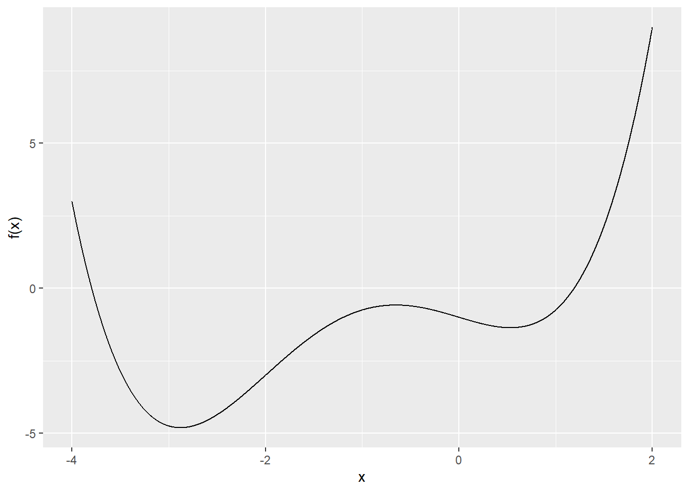
}Example: Find the local minima of \(f(x) = \frac{1}{4} x^4 + x^3 - x - 1\).
Plot:
Gradient descent:
f <- function(x) {1/4 * x^4 + x^3 - x - 1}
fp <- Deriv(f)

grad_des(fp, x0 = -2, h = 0.01)
## [1] -2.878224

grad_des(fp, x0 = 2, h = 0.01)
## [1] 0.5344022
Displaying error message:
grad_des(fp, x0 = -2, h = 0.01, max_iter = 2)
## Error in grad_des(fp, x0 = -2, h = 0.01, max_iter = 2): Maximum number of iterations reachedRemark: to find a local maximum, use gradient ascent.
Algorithm:
- Set an initial point \(x_0\) and a step size \(h > 0\)
- Iterate until convergence: \[\begin{equation*} x_{n+1} = x_{n} + h f'(x_{n}). \end{equation*}\]
Implementation:
grad_asc <- function(fp, x0, h = 1e-3, tol = 1e-4, max_iter = 1000) {
  grad_des(fp, x0, -h, tol, max_iter)
}
Example:
8.4 optim
optim() is a general-purpose optimization function in R. By default, it will try to minimize a function.
Basic Usage
Inputs:
par: initial values for the parameters to be opimtized overfn: a function to be minimized
Outputs:
par: the minimizervalue: the minimum value of the functionconvergence:0indicates successful completion
Example 1:
f <- function(x) {
  x^2 + 2*x + 1
}

fit <- optim(par = runif(1), fn = f)
fit
## $par
## [1] -0.9999646
##
## $value
## [1] 1.252847e-09
##
## $counts
## function gradient
##       36       NA
##
## $convergence
## [1] 0
##
## $message
## NULL
I used some random numbers for the initial values in optim() because we do not know a good estimate of the minimizer. In general, you will perform the optimization with several set of different initial values and see which one results in a smaller function value. Sometimes, the algorithm will get stuck in a local minimum and using several set of random initial values can alleviate this problem.
If you start at different initial values, you may get slightly different results
Example 2 (Multivariable function)
f <- function(x) {
  (x[1] - 2)^2 + (x[2] - 1)^2 + (x[3] + 3)^2
}

fit <- optim(par = c(0, 0, 0), fn = f)
fit
## $par
## [1]  2.0000917  0.9998627 -3.0002115
##
## $value
## [1] 7.20075e-08
##
## $counts
## function gradient
##      104       NA
##
## $convergence
## [1] 0
##
## $message
## NULL
Example 3 (Multivariable function where some of the variables are fixed)
f <- function(x, a) {
  (x[1] - a)^2 + (x[2] - 1)^2 + (x[3] + 3)^2
}

# provide the additional value of a
fit <- optim(par = c(0, 0, 0), fn = f, a = 5)
fit
## $par
## [1]  5.0001872  0.9999366 -3.0001587
##
## $value
## [1] 6.426168e-08
##
## $counts
## function gradient
##      128       NA
##
## $convergence
## [1] 0
##
## $message
## NULL
Example 4 (Setting box constraints on the parameters)
The Method “L-BFGS-B” allows box constraints, that is each variable can be given a lower and/or upper bound.
f <- function(x) {
  (x[1] - 2)^2 + (x[2] - 1)^2 + (x[3] + 3)^2
}

fit <- optim(par = c(0, 0, 0), fn = f, method = "L-BFGS-B",
             lower = c(-5, 0, 0), upper = c(1.5, 4, 5))
fit
## $par
## [1] 1.5 1.0 0.0
##
## $value
## [1] 9.25
##
## $counts
## function gradient
##        7        7
##
## $convergence
## [1] 0
##
## $message
## [1] "CONVERGENCE: NORM OF PROJECTED GRADIENT <= PGTOL"
To control the number of maximum iterations, add control = list(maxit = ...).
Small number of iterations may not lead to a converged solution
optim(par = c(0, 0, 0), fn = f, control = list(maxit = 10))
## $par
## [1]  0.33333333  0.03333333 -0.33333333
##
## $value
## [1] 10.82333
##
## $counts
## function gradient
##       12       NA
##
## $convergence
## [1] 1
##
## $message
## NULL
BFGS is a quasi-Newton method and usually converges quickly