Chapter 20 Evaluating Model Performance
Packages used in this chapter:
20.1 Accuracy and Confusion Matrix
We have defined Accuracy as
\[\begin{equation*} \text{Accuracy} = \frac{\text{number of correct predictions}}{\text{total number of predictions}}. \end{equation*}\]
However, the class imbalance problem below will show that this measure may not be a good measure of model performance in many cases.
Class imbalance problem
If you have a model with \(99\%\) accuracy, does that mean the model is useful?
Imagine a disease that is found 11 out of every 1000 people.
A model that predicts no disease will have an accuracy of \(989/1000 = 98.9\%\), which is just slightly lower than the accuracy of your model.
This shows that accuracy alone may not be a particular useful measure of performance in many applications.
Class imbalance problem = the trouble associated with data having a large majority of records belonging to a single class
Another problem is that accuracy does not tell us whether the model is good at identifying the positive cases or the negative cases.
Additionally, the consequence of having false negatives can be more severe than having false positives.
Confusion matrices
We have already seen some confusion matrices in previous chapters.
A confusion matrix is a table that categorizes predictions according to whether they match the actual value.
Correct predictions fall on the diagonal in the confusion matrix
Recall the logistic regression example:
library(mlbench)

data(PimaIndiansDiabetes2)
PimaIndiansDiabetes2 <- na.omit(PimaIndiansDiabetes2)

# Split the data into training and test set
set.seed(1)
random_index <- sample(nrow(PimaIndiansDiabetes2),
                       size = nrow(PimaIndiansDiabetes2) * 0.7)
train_data  <- PimaIndiansDiabetes2[random_index, ]
test_data <- PimaIndiansDiabetes2[-random_index, ]
fit_simple <- glm(diabetes ~ glucose, data = train_data, family = binomial)

# Prediction
prob <- predict(fit_simple, test_data, type = "response")
predicted_class <- ifelse(prob > 0.5, "pos", "neg")
We can use the function CrossTable() from the package gmodels to create a confusion matrix with some additional information.
library(gmodels)
CrossTable(predicted_class, test_data$diabetes, prop.chisq = FALSE)
##
##
##    Cell Contents
## |-------------------------|
## |                       N |
## |           N / Row Total |
## |           N / Col Total |
## |         N / Table Total |
## |-------------------------|
##
##
## Total Observations in Table:  118
##
##
##                 | test_data$diabetes
## predicted_class |       neg |       pos | Row Total |
## ----------------|-----------|-----------|-----------|
##             neg |        71 |        23 |        94 |
##                 |     0.755 |     0.245 |     0.797 |
##                 |     0.899 |     0.590 |           |
##                 |     0.602 |     0.195 |           |
## ----------------|-----------|-----------|-----------|
##             pos |         8 |        16 |        24 |
##                 |     0.333 |     0.667 |     0.203 |
##                 |     0.101 |     0.410 |           |
##                 |     0.068 |     0.136 |           |
## ----------------|-----------|-----------|-----------|
##    Column Total |        79 |        39 |       118 |
##                 |     0.669 |     0.331 |           |
## ----------------|-----------|-----------|-----------|
##
##
The \(3\) proportions are
- N / Row Total (e.g. \(71/94 = 0.755\))
- N / Col Total (e.g. \(71/79 = 0.899\))
- N / Table Total (e.g. \(71/118 = 0.602\))
In a confusion matrix, predictions fall into one of the four categories:
- True positive (TP): Correctly classified as the class of interest
- True negative (TN): Correctly classified as not the class of interest
- False positive (FP): Incorrectly classified as the class of interest
- False negative (FN): Incorrectly classified as not the class of interest
Positive = the class of interest
The notations TP, TN, FP and FN are also used to refer to the number of times the predictions fell into each of these categories.
In the logistic regression example, suppose our class of interest is pos.
- TP = 16
- TN = 71
- FP = 8
- FN = 23
20.2 Other Measures of Performance
The package caret contains a function confusionMatrix() to output several useful measures of classification performance. We will talk about some of them in the next section.
library(caret)
# requires factor inputs
confusionMatrix(data = factor(predicted_class), reference =  factor(test_data$diabetes),
                positive = "pos")
## Confusion Matrix and Statistics
##
##           Reference
## Prediction neg pos
##        neg  71  23
##        pos   8  16
##
##                Accuracy : 0.7373
##                  95% CI : (0.6483, 0.814)
##     No Information Rate : 0.6695
##     P-Value [Acc > NIR] : 0.06908
##
##                   Kappa : 0.3423
##
##  Mcnemar's Test P-Value : 0.01192
##
##             Sensitivity : 0.4103
##             Specificity : 0.8987
##          Pos Pred Value : 0.6667
##          Neg Pred Value : 0.7553
##              Prevalence : 0.3305
##          Detection Rate : 0.1356
##    Detection Prevalence : 0.2034
##       Balanced Accuracy : 0.6545
##
##        'Positive' Class : pos
##
20.2.1 The kappa statistic
Idea: we want to adjust accuracy by accounting for the possibility of a correct prediction by chance alone. For example, if the disease is found \(11\) out of every \(1000\) people, we can predict each case randomly by assigning the positive case with probability \(0.989\). In this way, our accuracy will be \(98.9\%\) on average.
Definition of the kappa statistic:
\[\begin{equation*} \kappa = \frac{p_a - p_e}{1 - p_e}, \end{equation*}\] where
- \(p_a\) is the proportion of actual agreement. That is, \(p_a\) is the proportion of all instances where the predicted type and actual type agree. Mathematically,
\[\begin{equation*} p_a = \frac{TP + TN}{TP + TN + FP + FN} = \text{Accuracy}. \end{equation*}\]
\(p_e\) is the expected agreement between the classifier and the true values, under the assumption that they were chosen at random. Let
\(p_{\text{pos, actual}}\) denote the proportion of the positive cases in the actual data
\(p_{\text{neg, actual}}\) denote the proportion of the negative cases in the actual data
\(p_{\text{pos, pred}}\) denote the proportion of the positive cases in the predictions
\(p_{\text{neg, pred}}\) denote the proportion of negative cases in the predictions
Mathematically,
\[\begin{equation*} p_e = p_{\text{pos, actual}} \times p_{\text{pos, pred}} + p_{\text{neg, actual}} \times p_{\text{neg, pred}}. \end{equation*}\] This is because there are only two ways to get agreement (both are positive and both are negative) and the predictions are chosen at random (so that the predictions and the actual data are independent -> independence means multiplication in probability).
In the above example,
- \(p_a = \frac{16 + 71}{118} = 0.7372881\)
- \(p_e = \frac{79}{118} \frac{94}{118} + \frac{39}{118} \frac{24}{118} = 0.6005458\).
- \(\kappa = \frac{p_a - p_e}{1 - p_e} = 0.342\).
Common interpretation of \(\kappa\):
- less than \(0.2\) = poor agreement
- \(0.2\) to \(0.4\) = fair agreement
- \(0.4\) to \(0.8\) = moderate agreement
- \(0.6\) to \(0.8\) = good agreement
- \(0.8\) to \(1\) = very good agreement
20.2.2 Sensitivity and specificity
Most of you have probably received some spam (junk email) in your email. Many email providers filter the spam automatically. You may also experience that sometimes some legitimate emails (ham) are classified as spam.
Finding a useful classifier often involves a balance between predictions that are overly conservative and overly aggressive.
(Overly Aggressive) For example, you can classify an email as spam if you have never sent an email to that address.
(Overly Conservative) To guarantee that no ham messages will be inadvertently filtered might require us to allow an unacceptable amount of spam to pass through the filter.
A pair of performance measures captures this trade-off: sensitivity and specificity.
Sensitivity (also called the true positive rate) is defined as \[\begin{equation*} \text{Sensitivity} = \frac{TP}{TP + FN}. \end{equation*}\] It is the proportion of positive examples that are correctly classified. E.g., the proportion of spam filtered.
Specificity (also called the true negative rate) is defined as \[\begin{equation*} \text{Specificity} = \frac{TN}{TN + FP}. \end{equation*}\] It is the proportion of negative examples that are correctly classified. E.g., the proportion of ham not filtered.
Ideally, we want both of them to be close to \(1\).
There is usually a tradeoff between the two measures.
20.2.3 Precision and Recall
Precision = positive predictive value = proportion of positive examples that are truly positive
Recall = sensitivity = number of true positives / total number of positives
20.2.4 ROC and AUC
ROC = receiver operating characteristic curve
AUC = area under the ROC curve
Recall that in the logistic regression example, we chose \(0.5\) as the threshold to decide our predictions. Changing this threshold will change the sensitivity and the specificity of your model. ROC is a tool to visualize the trade-off between the sensitivity and specificity. In ROC, sensitivity is plot against 1 - specificity at different levels of the threshold. It tells you how well the model perform.
- A classifier that is closer to the perfect classifier is considered to be better
- A classifier that results in a higher AUC is considered to be better
- The diagonal line from the bottom-left to the top-right corner of the diagram represents a classifier with no predictive value.
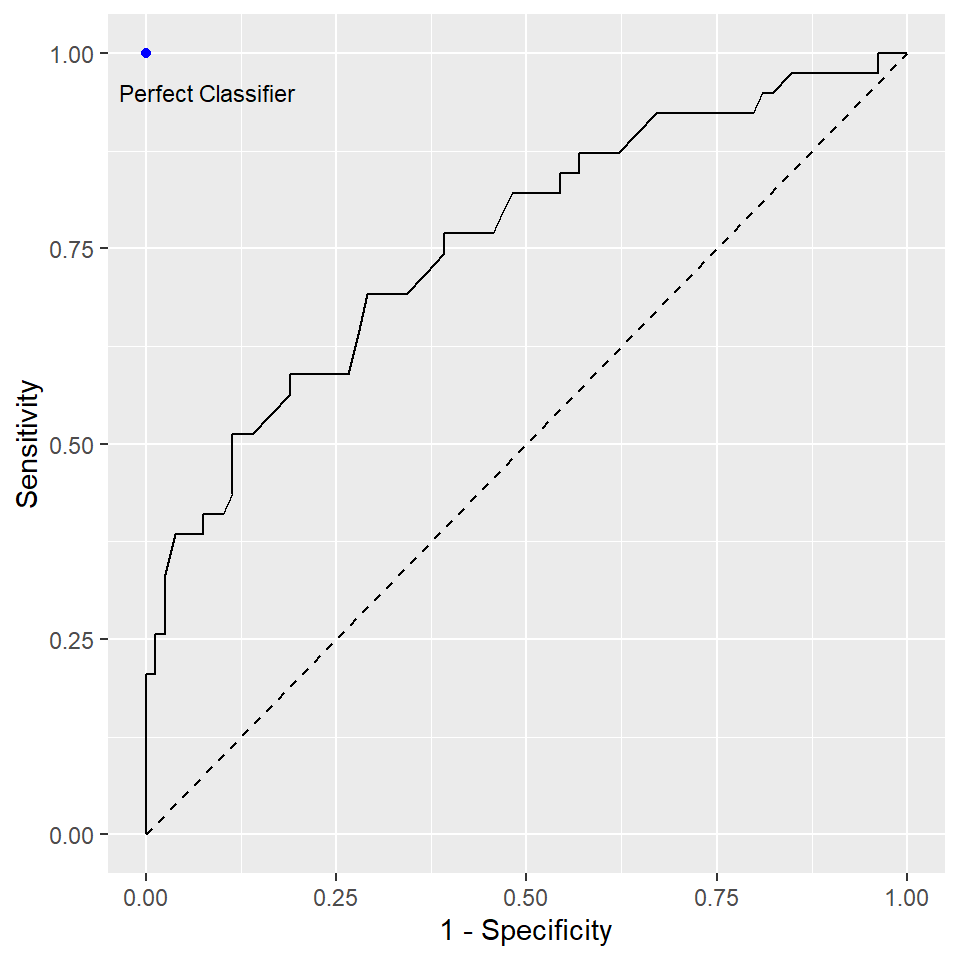
To understand how ROC is constructed, we use our logistic regression example. The package caret contains the two functions sensitivity and specificity to compute the sensitivity and specificity, respectively. The following code is used to create the above figure (without the dot corresponding to the perfect classifier).
library(caret)
threshold <- seq(0, 1, by = 0.001)
roc_sensitivity <- rep(0, length(threshold))
roc_specificity <- rep(0, length(threshold))

for (i in 1:length(threshold)) {
  # for each value of threshold, find our predictions
  predicted_class <- factor(ifelse(prob > threshold[i], "pos", "neg"))
  # compute the corresponding sensitivity and specificity
  roc_sensitivity[i] <- sensitivity(predicted_class, test_data$diabetes, positive = "pos")
  roc_specificity[i]  <- specificity(predicted_class, test_data$diabetes, negative = "neg")
}

# ROC, use geom_path instead of geom_line to retain the order when joining the points
ggplot(mapping = aes(x = 1 - roc_specificity, y = roc_sensitivity)) +
  geom_path() +
  labs(x = "1 - Specificity", y = "Sensitivity") +
  geom_segment(aes(x = 0, xend = 1, y = 0, yend = 1), linetype = 2)
There is a function called roc() in the package pROC to construct the ROC.
library(pROC)

roc_logistic <- roc(predictor = as.numeric(prob), response = test_data$diabetes)

plot(roc_logistic)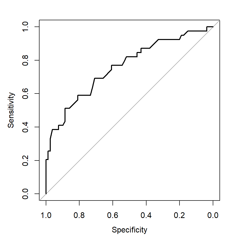
Note that the x-axis label from this function is Specificity starting from 1.
AUC values:
- 0.9-1.0: outstanding
- 0.8-0.9: excellent/good
- 0.7-0.8: acceptable/fair
- 0.6-0.7: poor
- 0.5-0.6: no discrimination power
20.3 Estimating future performances
Recall that in evaluating the model performance, we have partition our data into training and testing datasets. This is known as the holdout method.
To estimate the future performance, we should not use any part of the testing data when we train our model using our training dataset. Otherwise, our result will be biased.
One problem with the above random partition is that the proportions of the class of interest are very different in the training dataset and testing datase even if we have randomly selected our observations.
Example
set.seed(2)
random_index <- sample(nrow(PimaIndiansDiabetes2),
                       size = nrow(PimaIndiansDiabetes2) * 0.7)
train_data  <- PimaIndiansDiabetes2[random_index, ]
test_data <- PimaIndiansDiabetes2[-random_index, ]

table(train_data$diabetes) / nrow(train_data)
##
##      neg      pos
## 0.649635 0.350365

table(test_data$diabetes) / nrow(test_data)
##
##       neg       pos
## 0.7118644 0.2881356
You can see that the proportion of pos in the training dataset is \(0.350\) while that in the testing dataset is \(0.288\). This may affect the estimation of the model performance.
To avoid this issue, we can use stratified random sampling to ensure the training dataset and testing dataset have nearly the same proportion in the class of interest.
To do that in R, we can use the function createDataPartition from the package caret.
stratified_random_index <- createDataPartition(PimaIndiansDiabetes2$diabetes,
                                               p = 0.7, list = FALSE)

train_data  <- PimaIndiansDiabetes2[stratified_random_index, ]
test_data <- PimaIndiansDiabetes2[-stratified_random_index, ]

table(train_data$diabetes) / nrow(train_data)
##
##       neg       pos
## 0.6690909 0.3309091

table(test_data$diabetes) / nrow(test_data)
##
##       neg       pos
## 0.6666667 0.3333333

table(PimaIndiansDiabetes2$diabetes) / nrow(PimaIndiansDiabetes2)
##
##       neg       pos
## 0.6683673 0.3316327
Now, both proportions are similar to the one in the whole dataset.
While stratified sampling distribute the classes evenly, it does not guarantee other variables are distributed evenly.
- To mitigate the problem, we can use repeated holdout. That is, we repeat the whole process several times with several random holdout samples and take the average of the performance measures to evaluate the model performance. As multiple holdout samples are used, it is less likely that the model is trained or tested on non-representative data.
20.3.1 Cross-validation
\(k\)-fold cross-validation (\(k\)-fold CV) is a procedure in which instead of randomly partition the data many times, we divide the data into \(k\) random non-overlapping partitions. Then, we combine \(k-1\) partitions to form a training dataset and the remaining one to form the testing dataset. We repeat this procedure \(k\) times using different partitions and obtain \(k\) evaluations. It is common to use \(10\)-fold CV.
For example, when \(k=3\):
- Randomly split your dataset \(S\) into \(3\) partitions \(S_1,S_2,S_3\).
- Use \(S_1, S_2\) to train your model. Evaluate the performance using \(S_3\).
- Use \(S_1, S_3\) to train your model. Evaluate the performance using \(S_2\).
- Use \(S_2, S_3\) to train your model. Evaluate the performance using \(S_1\).
- Report the average of the performance measures obtained in Steps 2-4.
See https://en.wikipedia.org/wiki/File:KfoldCV.gif for a gif animation showing the \(k\)-fold CV.
Example:
k <- 10
set.seed(1)
# the result is a list
folds <- createFolds(PimaIndiansDiabetes2$diabetes, k = k)
accuracy <- rep(0, k)
AUC <- rep(0, k)

for (i in 1:k) {
  train_data  <- PimaIndiansDiabetes2[folds[[i]], ]
  test_data <- PimaIndiansDiabetes2[-folds[[i]], ]
  fit_simple <- glm(diabetes ~ glucose, data = train_data, family = binomial)

  # Prediction
  prob <- predict(fit_simple, test_data, type = "response")
  predicted_class <- ifelse(prob > 0.5, "pos", "neg")

  # Compute accuracy and AUC
  accuracy[i] <- mean(predicted_class == test_data$diabetes)
  AUC[i] <- auc(roc(predictor = as.numeric(prob), response = test_data$diabetes))
}
Results:
20.4 Class Imbalance in Classification
Class imbalance is a common problem in classification where one class (the minority class) has significantly fewer samples than another class (the majority class). This can lead to a biased model that favors the majority class, resulting in poor performance for the minority class. Here are some examples of class imbalance problems in classification:
Fraud Detection: In a credit card transaction dataset, the number of fraudulent transactions is much lower than the number of legitimate transactions.
Medical Diagnosis: In a medical diagnosis dataset, the number of positive cases for a rare disease is much lower than the number of negative cases.
Anomaly Detection: In an anomaly detection dataset, the number of anomalous data points is much lower than the number of normal data points.
Image Classification: In an image classification dataset, the number of images containing rare objects or events is much lower than the number of images containing common objects or events.
One popular method to deal wit in classification problems is the SMOTE (Synthetic Minority Over-sampling Technique) algorithm. It works by generating synthetic samples for the minority class, which can help balance the class distribution and improve the performance of the model.
SMOTE
Randomly select an instance from the minority class.
Randomly select one of the \(k\) nearest neighbors of the selected instance and create a new synthetic instance along the line segment between the selected instance and the chosen neighbor (In this way, the data will not be duplicated but slightly different from the original data.). The class label of the synthetic instance is the same as the minority class.
Repeat this process until the desired number of synthetic samples has been generated.
Download the archived version of DMwR here: https://cran.r-project.org/src/contrib/Archive/DMwR/
You may need to install the package ROCR first. Then, you can install DMwR by clicking Tools -> Install Packages -> Install from: Package archive file -> Browse: choose the file you downloaded above.
library(DMwR)

# simulated data set
set.seed(362)
n <- 1000
beta_0 <- c(-1, -1, -1) # true beta
x1 <- runif(n, 0, 1)
x2 <- runif(n, 0, 1)
prob_num <- exp(beta_0[1] + beta_0[2] * x1 + beta_0[3] * x2)
prob <- prob_num / (1 + prob_num)
y <- factor(rbinom(n, size = 1, prob = prob)) # the class has to be "factor"
data <- data.frame(y, x1, x2)

# SMOTE
new_data <- SMOTE(y ~ ., data, perc.over = 500, perc.under = 200)Note: Do not generate synthetic data in the test data.