Chapter 4 Managing Data with R

Reference: see https://r4ds.had.co.nz/transform.html

Optional Reading: ML with R Ch2

4.1 Missing Values

Missing values are common in real datasets.

NA is used to denote missing values.

(x <- c(1, 2, 3, NA, 4, NA, 4)) # we can use (x<-1) to assign 1 to x and display x at the same time
## [1]  1  2  3 NA  4 NA  4

mean(x) # mean cannot be computed when missing values exist
## [1] NA

mean(x, na.rm = TRUE) # NA values will be removed before computing mean
## [1] 2.8

sd(x)  # sd cannot be computed when missing values exist
## [1] NA

sd(x, na.rm = TRUE) # NA values will be removed before computing SD
## [1] 1.30384

is.na(x) # logical vector
## [1] FALSE FALSE FALSE  TRUE FALSE  TRUE FALSE

x[!is.na(x)] #select the elements with non-missing valuess
## [1] 1 2 3 4 4

na.omit(x) # select the elements with non-missing valuess
## [1] 1 2 3 4 4
## attr(,"na.action")
## [1] 4 6
## attr(,"class")
## [1] "omit"

4.2 Saving, loading, and removing R data structures

Removing all objects in R:

rm(list = ls())

ls() returns a vector of all data structures currently in memory

x <- c(1, 2, 3)
y <- c(4, 5, 6)
ls()
## [1] "x" "y"

To remove x from the memory

rm(x)
x # because we have deleted x, an error message occurs
## Error in eval(expr, envir, enclos): object 'x' not found

Saving objects to a file (regardless of whether they are vectors, factors, lists, etc)

A <- matrix(1:9, 3, 3)

f <- function(x){
  return(1)
}

save(A, f, file = "my_data.RData")

Loading objects from a .RData file.

rm(list = ls()) # remove everything 

load("my_data.RData")

A
##      [,1] [,2] [,3]
## [1,]    1    4    7
## [2,]    2    5    8
## [3,]    3    6    9

f
## function(x){
##   return(1)
## }

4.3 Importing and saving data from CSV files

Finding current directory

getwd()
## [1] "C:/Queens Teaching/01_Teaching/STAT 362 W24 R for data science/01c_published_webiste"

If you use mac, you will probably see "/Users/..../".

Setting working directory

setwd("C:/Queens Teaching/01_Teaching/STAT 362 W24 R for data science/01_lect_notes/Ch4_Managing_Data_and_dplyr") # use /, not \

If you use mac, change the above code accordingly.

Writing to a file

my_data <- data.frame(x = c(5, 10, 3), y = c(4, 5, 6))
my_data
##    x y
## 1  5 4
## 2 10 5
## 3  3 6
write.csv(my_data, "C:/Queens Teaching/01_Teaching/STAT 362 W24 R for data science/01_lect_notes/Ch4_Managing_Data_and_dplyr/my_data.csv", row.names = FALSE)

Reading a csv file

A comma-separated values (CSV) file is a delimited text file that uses a comma to separate values. If we use read_csv from the package tidyverse, the resulting object is a tibble. If we use read.csv from base R, the resulting object is a data frame. See R for data science (https://r4ds.had.co.nz/data-import.html) for a discussion on the differences between read.csv and read_csv.

my_data <- read.csv("C:/Queens Teaching/01_Teaching/STAT 362 W24 R for data science/01_lect_notes/Ch4_Managing_Data_and_dplyr/my_data.csv")

4.4 Data Transformation with `dplyr`

Preparation

We will use a dataset in the package nycflights13. To install it:

install.packages("nycflights13")

To use the dataset or functions in the package, we first load the library:

library(nycflights13)

In Chapter 4, we have installed tidyverse, which contains the package dplyr. Now, load the package

library(tidyverse)

nycflights13

The dataset flights in the package nyclfights13 contains all $336,776$ flights that departed from New York City in 2013. Check ?flights for details.

# let's view the dataset
flights
## # A tibble: 336,776 × 19
##     year month   day dep_time sched_dep_time dep_delay arr_time sched_arr_time arr_delay carrier flight tailnum origin dest  air_time distance  hour
##    <int> <int> <int>    <int>          <int>     <dbl>    <int>          <int>     <dbl> <chr>    <int> <chr>   <chr>  <chr>    <dbl>    <dbl> <dbl>
##  1  2013     1     1      517            515         2      830            819        11 UA        1545 N14228  EWR    IAH        227     1400     5
##  2  2013     1     1      533            529         4      850            830        20 UA        1714 N24211  LGA    IAH        227     1416     5
##  3  2013     1     1      542            540         2      923            850        33 AA        1141 N619AA  JFK    MIA        160     1089     5
##  4  2013     1     1      544            545        -1     1004           1022       -18 B6         725 N804JB  JFK    BQN        183     1576     5
##  5  2013     1     1      554            600        -6      812            837       -25 DL         461 N668DN  LGA    ATL        116      762     6
##  6  2013     1     1      554            558        -4      740            728        12 UA        1696 N39463  EWR    ORD        150      719     5
##  7  2013     1     1      555            600        -5      913            854        19 B6         507 N516JB  EWR    FLL        158     1065     6
##  8  2013     1     1      557            600        -3      709            723       -14 EV        5708 N829AS  LGA    IAD         53      229     6
##  9  2013     1     1      557            600        -3      838            846        -8 B6          79 N593JB  JFK    MCO        140      944     6
## 10  2013     1     1      558            600        -2      753            745         8 AA         301 N3ALAA  LGA    ORD        138      733     6
## # ℹ 336,766 more rows
## # ℹ 2 more variables: minute <dbl>, time_hour <dttm>

flights is a tibble. Tibbles are data frames with better properties.

Optional: If you are interested in the differences between a data frame and a tibble, you can go to https://cran.r-project.org/web/packages/tibble/vignettes/tibble.html

To view the complete dataset, use View(flights).

Five key dplyr functions

arrange(): reorder the rows
fliter(): pick observations by their values
select(): pick variables by their names
mutate(): create new variables with functions of existing variables
summarize(): collapse many values down to a single summary

All functions work similarly:

The first argument is a data frame/ tibble
The subsequent argument describe what to do with the data frame, using the variable names (without quotes).
The result is a new data frame.

Of course, it is also possible to perform the same tasks without using dplyr functions. We will also discuss briefly how to use the base subsetting with [] to select the data. In general, the functions in dplyr are designed to transform the data more easily.

4.5 `arrange()`

arrange() orders your dataset. If more than one column name is provided, each additional column will be used to break ties in the values of preceding columns.

To reorder by a column in ascending order:

arrange(flights, year, month, day)

Let’s create a simple dataset to illustrate this because flights is already sorted in year, month and day.

(data <- tibble(x = c(2, 2, 1, 4, 5), y = c(2, 3, 10, 10, 10)))
## # A tibble: 5 × 2
##       x     y
##   <dbl> <dbl>
## 1     2     2
## 2     2     3
## 3     1    10
## 4     4    10
## 5     5    10

arrange(data, x)
## # A tibble: 5 × 2
##       x     y
##   <dbl> <dbl>
## 1     1    10
## 2     2     2
## 3     2     3
## 4     4    10
## 5     5    10

# first sort in ascending order of x, use y to break any ties and sort in descending order
arrange(data, x, desc(y))
## # A tibble: 5 × 2
##       x     y
##   <dbl> <dbl>
## 1     1    10
## 2     2     3
## 3     2     2
## 4     4    10
## 5     5    10

To reorder by a column in descending order, use desc():

arrange(flights, desc(arr_delay))

Missing values are always sorted at the end

# create a tibble with one column called x with values 5,2,NA
df <- tibble(x = c(5, 2, NA)) 
arrange(df, x)
## # A tibble: 3 × 1
##       x
##   <dbl>
## 1     2
## 2     5
## 3    NA

arrange(df, desc(x))
## # A tibble: 3 × 1
##       x
##   <dbl>
## 1     5
## 2     2
## 3    NA

4.5.1 Exercises

Sort flights to find the most delayed flights. Find the flights that left earliest.

arrange(flights, desc(dep_delay))

arrange(flights, dep_delay)

Which flights traveled the longest? Which traveled the shortest?

arrange(flights, desc(distance))

arrange(flights, distance)

4.6 `filter()`

filter() only includes rows where the condition is TRUE

Select all flights on Jan 1st:

# flights is the name of your data frame
# month == 1, day == 1 is the condition
(jan1 <- filter(flights, month == 1, day == 1))
## # A tibble: 842 × 19
##     year month   day dep_time sched_dep_time dep_delay arr_time sched_arr_time arr_delay carrier flight tailnum origin dest  air_time distance  hour
##    <int> <int> <int>    <int>          <int>     <dbl>    <int>          <int>     <dbl> <chr>    <int> <chr>   <chr>  <chr>    <dbl>    <dbl> <dbl>
##  1  2013     1     1      517            515         2      830            819        11 UA        1545 N14228  EWR    IAH        227     1400     5
##  2  2013     1     1      533            529         4      850            830        20 UA        1714 N24211  LGA    IAH        227     1416     5
##  3  2013     1     1      542            540         2      923            850        33 AA        1141 N619AA  JFK    MIA        160     1089     5
##  4  2013     1     1      544            545        -1     1004           1022       -18 B6         725 N804JB  JFK    BQN        183     1576     5
##  5  2013     1     1      554            600        -6      812            837       -25 DL         461 N668DN  LGA    ATL        116      762     6
##  6  2013     1     1      554            558        -4      740            728        12 UA        1696 N39463  EWR    ORD        150      719     5
##  7  2013     1     1      555            600        -5      913            854        19 B6         507 N516JB  EWR    FLL        158     1065     6
##  8  2013     1     1      557            600        -3      709            723       -14 EV        5708 N829AS  LGA    IAD         53      229     6
##  9  2013     1     1      557            600        -3      838            846        -8 B6          79 N593JB  JFK    MCO        140      944     6
## 10  2013     1     1      558            600        -2      753            745         8 AA         301 N3ALAA  LGA    ORD        138      733     6
## # ℹ 832 more rows
## # ℹ 2 more variables: minute <dbl>, time_hour <dttm>

Let’s use a simple dataset to see how to perform the same task without filter:

# just a simple dataset
(data <- tibble(x = c(1, 3, 5, 5, 3), y = 1:5))
## # A tibble: 5 × 2
##       x     y
##   <dbl> <int>
## 1     1     1
## 2     3     2
## 3     5     3
## 4     5     4
## 5     3     5

data$x == 5 # logical vector
## [1] FALSE FALSE  TRUE  TRUE FALSE

data[data$x == 5, ] # select the rows with value "TRUE"
## # A tibble: 2 × 2
##       x     y
##   <dbl> <int>
## 1     5     3
## 2     5     4

# returning to the flights dataset
base_jan1 <- flights[(flights$month == 1 & flights$day == 1), ]

(flights$month == 1 & flights$day == 1) is a logical vector indicating if the corresponding flight was on Jan 1 (TRUE if yes).

Now, let’s check if jan1 and base_jan1 are the same using identical:

identical(jan1, base_jan1) # TURE means they are the same, FALSE means they are not the same
## [1] TRUE

More Examples

Select flights that departed in Nov or Dec

filter(flights, month == 11 | month == 12)

# alternatively, simpler code
filter(flights, month %in% c(11, 12))

How to use the operator %in%?

y <- c(1,3,5)

x <- 1
x %in% y #whether 1 is in {1,3,5}
## [1] TRUE

x <- c(1,3,2,4,1)
x %in% y # check whether each element in x is in {1,3,5}
## [1]  TRUE  TRUE FALSE FALSE  TRUE

%in% also works with characters

c("a", "b") %in% c("a", "c", "d")
## [1]  TRUE FALSE

The result is TRUE FALSE because "a" is in c("a", "c", "d") and "b" is not in c("a", "c", "d").

Perform the same task without filter:

flights[flights$month == 11 | flights$month == 12,]

# or 
flights[flights$month %in% c(11, 12), ]

Flights that were not delayed (on arrival or departure) by more than two hours:

delay1 <- filter(flights, arr_delay <= 120, dep_delay <= 120)

Without using filter

delay2 <- flights[flights$arr_delay <= 120 & flights$dep_delay <= 120, ]

Let’s check if delay1 and delay2 are the same.

identical(delay1, delay2)
## [1] FALSE

The result is FALSE, meaning delay1 and delay2 are not the same. Why? Because some elements in flights$arr_delay <= 120 & flights$dep_delay <= 120 are NA.

# to find out the number of NA values
sum(is.na(flights$arr_delay <= 120 & flights$dep_delay <= 120))
## [1] 9304

As a result, with the base subsetting method, a row with all NA values will be selected. On the other hand, for filter, when a condition evaluates to NA, the row will be dropped. Let’s create a small dataset to illustrate this. From now on, let’s try to use tibble instead of data.frame.

data <- tibble(x = 1:4, y = c(1, 2, NA, 4)) 

data[data$y <= 3, ] 
## # A tibble: 3 × 2
##       x     y
##   <int> <dbl>
## 1     1     1
## 2     2     2
## 3    NA    NA

# to avoid the above problem
# which() returns which elements are TRUE
which(data$y <= 3) # the result is 1, 2
## [1] 1 2
data[which(data$y <= 3), ] # select row 1, row 2
## # A tibble: 2 × 2
##       x     y
##   <int> <dbl>
## 1     1     1
## 2     2     2

# using filter
filter(data, y <= 3)
## # A tibble: 2 × 2
##       x     y
##   <int> <dbl>
## 1     1     1
## 2     2     2

# if we want to include the row where the value of y is NA
# recall that | means "or"
data[which(data$y <= 3 | is.na(data$y)), ]
## # A tibble: 3 × 2
##       x     y
##   <int> <dbl>
## 1     1     1
## 2     2     2
## 3     3    NA

# using filter
filter(data, y <= 3 | is.na(y)) 
## # A tibble: 3 × 2
##       x     y
##   <int> <dbl>
## 1     1     1
## 2     2     2
## 3     3    NA

If you want to drop the NA values with base subsetting[], you may use

delay3 <- flights[which((flights$arr_delay <= 120 & flights$dep_delay <= 120) == TRUE), ]

To see if delay1 and delay3 are exactly the same:

identical(delay1, delay3) # TRUE means exactly the same
## [1] TRUE

At this point, you should see that filter could perform the same tasks with simpler code.

4.6.1 Exercises

1a. Find all flights that had an arrival delay of two or more hours (drop the rows with NA in arr_delay).

# Using "filter"
filter(flights, arr_delay >= 120)

# Without using "filter"
flights[which(flights$arr_delay >= 120), ]

1b. Find all flights that flew to Houston (IAH or HOU).

# Using "filter"
filter(flights, dest %in% c("IAH", "HOU"))

# Without using "filter"
flights[which(flights$dest %in% c("IAH", "HOU")), ]

1c. Find all flights that were operated by United, American, or Delta

# find all the sorted carrier codes in the dataset
sort(unique(flights$carrier)) 
##  [1] "9E" "AA" "AS" "B6" "DL" "EV" "F9" "FL" "HA" "MQ" "OO" "UA" "US" "VX" "WN" "YV"

# look up airline names from their carrier codes
airlines 
## # A tibble: 16 × 2
##    carrier name                       
##    <chr>   <chr>                      
##  1 9E      Endeavor Air Inc.          
##  2 AA      American Airlines Inc.     
##  3 AS      Alaska Airlines Inc.       
##  4 B6      JetBlue Airways            
##  5 DL      Delta Air Lines Inc.       
##  6 EV      ExpressJet Airlines Inc.   
##  7 F9      Frontier Airlines Inc.     
##  8 FL      AirTran Airways Corporation
##  9 HA      Hawaiian Airlines Inc.     
## 10 MQ      Envoy Air                  
## 11 OO      SkyWest Airlines Inc.      
## 12 UA      United Air Lines Inc.      
## 13 US      US Airways Inc.            
## 14 VX      Virgin America             
## 15 WN      Southwest Airlines Co.     
## 16 YV      Mesa Airlines Inc.

# after looking up the names, we know UA = United, AA = American, DL = Delta
filter(flights, carrier %in% c("UA", "AA", "DL"))
## # A tibble: 139,504 × 19
##     year month   day dep_time sched_dep_time dep_delay arr_time sched_arr_time arr_delay carrier flight tailnum origin dest  air_time distance  hour
##    <int> <int> <int>    <int>          <int>     <dbl>    <int>          <int>     <dbl> <chr>    <int> <chr>   <chr>  <chr>    <dbl>    <dbl> <dbl>
##  1  2013     1     1      517            515         2      830            819        11 UA        1545 N14228  EWR    IAH        227     1400     5
##  2  2013     1     1      533            529         4      850            830        20 UA        1714 N24211  LGA    IAH        227     1416     5
##  3  2013     1     1      542            540         2      923            850        33 AA        1141 N619AA  JFK    MIA        160     1089     5
##  4  2013     1     1      554            600        -6      812            837       -25 DL         461 N668DN  LGA    ATL        116      762     6
##  5  2013     1     1      554            558        -4      740            728        12 UA        1696 N39463  EWR    ORD        150      719     5
##  6  2013     1     1      558            600        -2      753            745         8 AA         301 N3ALAA  LGA    ORD        138      733     6
##  7  2013     1     1      558            600        -2      924            917         7 UA         194 N29129  JFK    LAX        345     2475     6
##  8  2013     1     1      558            600        -2      923            937       -14 UA        1124 N53441  EWR    SFO        361     2565     6
##  9  2013     1     1      559            600        -1      941            910        31 AA         707 N3DUAA  LGA    DFW        257     1389     6
## 10  2013     1     1      559            600        -1      854            902        -8 UA        1187 N76515  EWR    LAS        337     2227     6
## # ℹ 139,494 more rows
## # ℹ 2 more variables: minute <dbl>, time_hour <dttm>

1d. Find all flights that departed in summer (July, August, and September)

filter(flights, month %in% c(7, 8, 9))

# Alternative Method
filter(flights, between(month, 7, 9))

1e. Find all flights that arrived more than two hours late, but didn’t leave late

filter(flights, arr_delay > 120, dep_delay <= 0)

The next two exercises are trickier.

1f. Find all flights that were delayed by at least an hour, but made up over 30 minutes in flight. First, the flight was delayed by at least an hour is the same as dep_delay >=60. Second, if a flight made up over 30 minutes in flight, the arrival delay must be at least 30 minutes less than the departure delay, which is the same as dep_delay - arr_delay > 30.

filter(flights, dep_delay >= 60, dep_delay - arr_delay > 30)

1g. Find all flights that departed between midnight and 6 a.m. (inclusive). The first question that should come to your mind is how is midnight represented in the dataset? Let’s take a look at summary(flights$dep_time).

summary(flights$dep_time)
##    Min. 1st Qu.  Median    Mean 3rd Qu.    Max.    NA's 
##       1     907    1401    1349    1744    2400    8255

The minimum is 1 and the maximum is 2400. Therefore, you know midnight is represented by 2400 instead of 0 in this dataset. The answer to the question would be

filter(flights, dep_time <= 600 | dep_time == 2400)

4.7 `select()`

Very often, we are only interested in some variables in a dataset. In that case, we can focus on the variables by creating a new dataset with those variables only. select() is to select the columns in a dataset by the name of the columns

Selecting Variables

Suppose you want to select the following $3$ columns in flights: year, month, day:

select(flights, year, month, day)
## # A tibble: 336,776 × 3
##     year month   day
##    <int> <int> <int>
##  1  2013     1     1
##  2  2013     1     1
##  3  2013     1     1
##  4  2013     1     1
##  5  2013     1     1
##  6  2013     1     1
##  7  2013     1     1
##  8  2013     1     1
##  9  2013     1     1
## 10  2013     1     1
## # ℹ 336,766 more rows

The usual way without using select() is

flights[c("year", "month", "day")] # or flights[, c("year", "month", "day")]
## # A tibble: 336,776 × 3
##     year month   day
##    <int> <int> <int>
##  1  2013     1     1
##  2  2013     1     1
##  3  2013     1     1
##  4  2013     1     1
##  5  2013     1     1
##  6  2013     1     1
##  7  2013     1     1
##  8  2013     1     1
##  9  2013     1     1
## 10  2013     1     1
## # ℹ 336,766 more rows

Select all columns between year and day (inclusive)

select(flights, year:day)
## # A tibble: 336,776 × 3
##     year month   day
##    <int> <int> <int>
##  1  2013     1     1
##  2  2013     1     1
##  3  2013     1     1
##  4  2013     1     1
##  5  2013     1     1
##  6  2013     1     1
##  7  2013     1     1
##  8  2013     1     1
##  9  2013     1     1
## 10  2013     1     1
## # ℹ 336,766 more rows

Excluding Variables

Select all columns except those from year to day (inclusive)

select(flights, -(year:day))

select(flights, -year, -month, -day)

Without using select()

flights[, !(colnames(flights) %in% c("year", "day", "month"))]

4.7.1 Exercises

You can also use

starts_with("abc") matches names that begin with "abc"
ends_with("xyz") matches names that end with "xyz"
contains("ijk") mathces names that contain "ijk"

Ex: select all columns that end with "delay".

select(flights, ends_with("delay"))
## # A tibble: 336,776 × 2
##    dep_delay arr_delay
##        <dbl>     <dbl>
##  1         2        11
##  2         4        20
##  3         2        33
##  4        -1       -18
##  5        -6       -25
##  6        -4        12
##  7        -5        19
##  8        -3       -14
##  9        -3        -8
## 10        -2         8
## # ℹ 336,766 more rows

Ex: select all columns that start with "a".

select(flights, starts_with("a"))
## # A tibble: 336,776 × 3
##    arr_time arr_delay air_time
##       <int>     <dbl>    <dbl>
##  1      830        11      227
##  2      850        20      227
##  3      923        33      160
##  4     1004       -18      183
##  5      812       -25      116
##  6      740        12      150
##  7      913        19      158
##  8      709       -14       53
##  9      838        -8      140
## 10      753         8      138
## # ℹ 336,766 more rows

Does the result of running the following code surprise you?

select(flights, contains("TIME"))
## # A tibble: 336,776 × 6
##    dep_time sched_dep_time arr_time sched_arr_time air_time time_hour          
##       <int>          <int>    <int>          <int>    <dbl> <dttm>             
##  1      517            515      830            819      227 2013-01-01 05:00:00
##  2      533            529      850            830      227 2013-01-01 05:00:00
##  3      542            540      923            850      160 2013-01-01 05:00:00
##  4      544            545     1004           1022      183 2013-01-01 05:00:00
##  5      554            600      812            837      116 2013-01-01 06:00:00
##  6      554            558      740            728      150 2013-01-01 05:00:00
##  7      555            600      913            854      158 2013-01-01 06:00:00
##  8      557            600      709            723       53 2013-01-01 06:00:00
##  9      557            600      838            846      140 2013-01-01 06:00:00
## 10      558            600      753            745      138 2013-01-01 06:00:00
## # ℹ 336,766 more rows

Yes, because we used “TIME” but not “time” and still get the selected columns. If you check ?contains, you can see that the default is to ignore the case. To change the default:

select(flights, contains("TIME", ignore.case = FALSE))
## # A tibble: 336,776 × 0

Ex: without using select(), select all the columns that contain “time”.

flights[grep("time", names(flights))]
## # A tibble: 336,776 × 6
##    dep_time sched_dep_time arr_time sched_arr_time air_time time_hour          
##       <int>          <int>    <int>          <int>    <dbl> <dttm>             
##  1      517            515      830            819      227 2013-01-01 05:00:00
##  2      533            529      850            830      227 2013-01-01 05:00:00
##  3      542            540      923            850      160 2013-01-01 05:00:00
##  4      544            545     1004           1022      183 2013-01-01 05:00:00
##  5      554            600      812            837      116 2013-01-01 06:00:00
##  6      554            558      740            728      150 2013-01-01 05:00:00
##  7      555            600      913            854      158 2013-01-01 06:00:00
##  8      557            600      709            723       53 2013-01-01 06:00:00
##  9      557            600      838            846      140 2013-01-01 06:00:00
## 10      558            600      753            745      138 2013-01-01 06:00:00
## # ℹ 336,766 more rows

Basic Usage of grep: grep(pattern, x).

pattern: character string. e.g., “time”, “delay”, “air”
x: a character vector where matches are sought. e.g., the colnames of a dataframe.
Output: a vector of the indices of the elements of x that yielded a match.

some_names <- c("ab", "bc", "cd")
grep("b", some_names)
## [1] 1 2
grep("d", some_names)
## [1] 3
grep("e", some_names)
## integer(0)

4.8 `mutate()`

Add new variables with mutate()

Very often, we want to create a new variable based on existing variables. For example, if we have distance and time, we can compute the speed by distance/time.

mutate() always adds new columns at the end of the dataset. Let’s create a narrower dataset so that we can see the result of mutate without use View().

# create a smaller dataset
flights_sml <- select(flights, year:day, arr_delay, dep_delay, distance, air_time)

Now, let’s use mutate() to create a variable called gain (how much time we gain in flight) defined as arr_delay - dep_delay and a variable called speed (miles/hour) defined as distance/air_time * 60.

mutate(flights_sml, gain = arr_delay - dep_delay, speed = distance / air_time * 60)
## # A tibble: 336,776 × 9
##     year month   day arr_delay dep_delay distance air_time  gain speed
##    <int> <int> <int>     <dbl>     <dbl>    <dbl>    <dbl> <dbl> <dbl>
##  1  2013     1     1        11         2     1400      227     9  370.
##  2  2013     1     1        20         4     1416      227    16  374.
##  3  2013     1     1        33         2     1089      160    31  408.
##  4  2013     1     1       -18        -1     1576      183   -17  517.
##  5  2013     1     1       -25        -6      762      116   -19  394.
##  6  2013     1     1        12        -4      719      150    16  288.
##  7  2013     1     1        19        -5     1065      158    24  404.
##  8  2013     1     1       -14        -3      229       53   -11  259.
##  9  2013     1     1        -8        -3      944      140    -5  405.
## 10  2013     1     1         8        -2      733      138    10  319.
## # ℹ 336,766 more rows

To keep the new variables only, use transmute():

transmute(flights_sml, gain = arr_delay - dep_delay, speed = distance /  air_time * 60)
## # A tibble: 336,776 × 2
##     gain speed
##    <dbl> <dbl>
##  1     9  370.
##  2    16  374.
##  3    31  408.
##  4   -17  517.
##  5   -19  394.
##  6    16  288.
##  7    24  404.
##  8   -11  259.
##  9    -5  405.
## 10    10  319.
## # ℹ 336,766 more rows

Without using select and mutate(), one may use

flights_sml2 <- flights[c("year", "month", "day", "arr_delay", "dep_delay", "distance", "air_time")]

flights_sml2$gain <- flights_sml2$arr_delay - flights_sml2$dep_delay

flights_sml2$speed <- flights_sml2$distance / flights_sml2$air_time * 60

4.8.1 Exercises

Ex: Currently, dep_time and sched_dep_time are convenient to look at, but hard to compute with because they are not really continuous numbers. Convert them to a more convenient representation of number of minutes since midnight.

Recall that dep_time and sched_dep_time are in HHMM format. For example, 1304 means 1:04pm. The number of minutes since midnight is $13\times 60 + 4 = 784$. In general, we can use the integer division to find the number of hours since midnight, then multiply by $60$, and finally add the remainder for the minutes. For example,

1304 %/% 100 # get the number of hours since midnight
## [1] 13

1304 %% 100 # get the remainder
## [1] 4

1304 %/% 100 * 60 + 1304 %% 100 # number of minutes since midnight
## [1] 784

Recall that midnight is represented as 2400 in the dataset and the number of minutes since midnight should be 0. However, if we use the above method for midnight, we get

2400 %/% 100 * 60 + 2400 %% 100 # this is not correct for midnight
## [1] 1440

Therefore, we also have to deal with this case. One possible solution is to do another integer division by 1440 (24x60 = 1440):

(1304 %/% 100 * 60 + 1304 %% 100) %% 1440 # will not change the result if the time is not midnight
## [1] 784

(2400 %/% 100 * 60 + 2400 %% 100) %% 1440 # this is correct for midnight
## [1] 0

Go back to flights:

# let's keep only the dep_time and sched_dep_time
flights_time <- select(flights, dep_time, sched_dep_time)

mutate(flights_time, min_dep_time = (dep_time %/% 100 * 60 + dep_time %% 100) %% 1440, 
       min_sched_dep_time = (sched_dep_time %/% 100 * 60 + sched_dep_time %% 100) %% 1440)
## # A tibble: 336,776 × 4
##    dep_time sched_dep_time min_dep_time min_sched_dep_time
##       <int>          <int>        <dbl>              <dbl>
##  1      517            515          317                315
##  2      533            529          333                329
##  3      542            540          342                340
##  4      544            545          344                345
##  5      554            600          354                360
##  6      554            558          354                358
##  7      555            600          355                360
##  8      557            600          357                360
##  9      557            600          357                360
## 10      558            600          358                360
## # ℹ 336,766 more rows

The above code doesn’t look good because we have written the formula to complete the same task twice. We can define a function to do this:

time_to_minutes <- function(x) {
  (x %/% 100 * 60 + x %% 100) %% 1440
}

With the function time_to_minutes, we have:

mutate(flights, min_dep_time = time_to_minutes(dep_time),
                min_sched_dep_time = time_to_minutes(sched_dep_time))

If you cannot think of using %% 1440 to deal with the midnight cases, we can write:

# ind for indicator approach
time_to_minutes_ind <- function(x) {
  (x %/% 100 * 60 + x %% 100) * (x != 2400)
}

# Explanation
# if x is 2400, (x!=2400) is FALSE, FALSE times a number y is 0
# if x is not 2400, (x!=2400) is TRUE, TRUE times a number y is y
# because "FALSE=0, TRUE=1"

mutate(flights, min_dep_time = time_to_minutes_ind(dep_time),
                min_sched_dep_time = time_to_minutes_ind(sched_dep_time))

An alternative way is to use ifelse (which is a vectorized function).

Usage of ifelse: ifelse(test, yes, no)

time_to_minutes_ifelse <- function(x) {
  ifelse(x != 2400, x %/% 100 * 60 + x %% 100, 0)  
}

mutate(flights, min_dep_time = time_to_minutes_ifelse(dep_time),
                min_sched_dep_time = time_to_minutes_ifelse(sched_dep_time))
## # A tibble: 336,776 × 21
##     year month   day dep_time sched_dep_time dep_delay arr_time sched_arr_time arr_delay carrier flight tailnum origin dest  air_time distance  hour
##    <int> <int> <int>    <int>          <int>     <dbl>    <int>          <int>     <dbl> <chr>    <int> <chr>   <chr>  <chr>    <dbl>    <dbl> <dbl>
##  1  2013     1     1      517            515         2      830            819        11 UA        1545 N14228  EWR    IAH        227     1400     5
##  2  2013     1     1      533            529         4      850            830        20 UA        1714 N24211  LGA    IAH        227     1416     5
##  3  2013     1     1      542            540         2      923            850        33 AA        1141 N619AA  JFK    MIA        160     1089     5
##  4  2013     1     1      544            545        -1     1004           1022       -18 B6         725 N804JB  JFK    BQN        183     1576     5
##  5  2013     1     1      554            600        -6      812            837       -25 DL         461 N668DN  LGA    ATL        116      762     6
##  6  2013     1     1      554            558        -4      740            728        12 UA        1696 N39463  EWR    ORD        150      719     5
##  7  2013     1     1      555            600        -5      913            854        19 B6         507 N516JB  EWR    FLL        158     1065     6
##  8  2013     1     1      557            600        -3      709            723       -14 EV        5708 N829AS  LGA    IAD         53      229     6
##  9  2013     1     1      557            600        -3      838            846        -8 B6          79 N593JB  JFK    MCO        140      944     6
## 10  2013     1     1      558            600        -2      753            745         8 AA         301 N3ALAA  LGA    ORD        138      733     6
## # ℹ 336,766 more rows
## # ℹ 4 more variables: minute <dbl>, time_hour <dttm>, min_dep_time <dbl>, min_sched_dep_time <dbl>

A less efficient way with for loop and if-else:

# if for if-else approach
time_to_minutes_if <- function(x) {
  n <- length(x)
  output <- rep(0, n)
  for (i in 1:n) {
    if (is.na(x[i])){ # check for NA
      output[i] <- NA
    } else if (x[i] != 2400) { # if not equal to 2400
      output[i] <- x[i] %/% 100 * 60 + x[i] %% 100
    } else { # if equal to 2400
      output[i] <- 0
    }
  }
  return(output)
}

mutate(flights, min_dep_time = time_to_minutes_if(dep_time),
                min_sched_dep_time = time_to_minutes_if(sched_dep_time))

Compare the efficiency:

system.time(mutate(flights, min_dep_time = time_to_minutes(dep_time),
                min_sched_dep_time = time_to_minutes(sched_dep_time)))
##    user  system elapsed 
##    0.03    0.00    0.04

system.time(mutate(flights, min_dep_time = time_to_minutes_if(dep_time),
                min_sched_dep_time = time_to_minutes_if(sched_dep_time)))
##    user  system elapsed 
##    0.00    0.00    0.18

4.9 `summarize(), group_by()`

Average delay over the year (not useful):

summarize(flights, delay = mean(dep_delay, na.rm = TRUE))
## # A tibble: 1 × 1
##   delay
##   <dbl>
## 1  12.6

Using summarize with group_by and ungroup can result in more useful statistics.

Use group_by. First argument is your dataset. Subsequent arguments indicate how you want to group the data.
In summarize, the dataset becomes the dataset from group_by.
After performing the calculation using summarize, use ungroup. If you do not use ungroup after group_by, the grouping structure is still retained in the object that you create and the subsequent calculation may yield something that you do not expect.

E.g.: Average departure delay per date (more useful):

by_day <- group_by(flights, year, month, day)
mean_delay <- summarize(by_day, delay = mean(dep_delay, na.rm = TRUE))
## `summarise()` has grouped output by 'year', 'month'. You can override using the `.groups` argument.
(mean_delay <- ungroup(mean_delay)) # use ungroup() after gropu_by()
## # A tibble: 365 × 4
##     year month   day delay
##    <int> <int> <int> <dbl>
##  1  2013     1     1 11.5 
##  2  2013     1     2 13.9 
##  3  2013     1     3 11.0 
##  4  2013     1     4  8.95
##  5  2013     1     5  5.73
##  6  2013     1     6  7.15
##  7  2013     1     7  5.42
##  8  2013     1     8  2.55
##  9  2013     1     9  2.28
## 10  2013     1    10  2.84
## # ℹ 355 more rows

4.10 Combining Multiple Operations with Pipe `%>%`

You can use the shortcut Ctrl/Cmd + Shift + M to insert the pipe operator %>%.

x %>% f(y) turns into f(x,y)

For example,

flights %>% 
  filter(month == 1, day == 1)

is the same as

filter(flights, month == 1, day == 1)

x %>% f(y) %>% g(z) turns into g(f(x,y),z).

For example,

flights %>% 
  group_by(year, month) %>% 
  summarize(mean_dep_delay = mean(dep_delay, na.rm = TRUE)) %>% 
  ungroup()

is the same as

ungroup(summarize(group_by(flights, year, month), mean_dep_delay = mean(dep_delay, na.rm = TRUE)))

Using the pipe can avoid creating and naming intermediate objects that we don’t need. Instead, the pipe focuses on the sequence of actions, not the object that the actions being performed on. It also tends to make the code easier to read. For the above example, you can read it as: for the dataset flights, we first group the data by year and month, then summarize the data by finding the mean. We can think of the pipe %>% as “then”.

Note: if you have to manipulate some intermediate objects, it may make sense not to use the pipe operator in that situation.

More examples:

Average delay per month:

by_month <- group_by(flights, month)
ungroup(summarize(by_month, delay = mean(dep_delay, na.rm = TRUE)))
## # A tibble: 12 × 2
##    month delay
##    <int> <dbl>
##  1     1 10.0 
##  2     2 10.8 
##  3     3 13.2 
##  4     4 13.9 
##  5     5 13.0 
##  6     6 20.8 
##  7     7 21.7 
##  8     8 12.6 
##  9     9  6.72
## 10    10  6.24
## 11    11  5.44
## 12    12 16.6

flights %>% 
  group_by(month) %>% 
  summarize(delay = mean(dep_delay, na.rm = TRUE)) %>% 
  ungroup() # a good habit is to use ungroup after the calculations
## # A tibble: 12 × 2
##    month delay
##    <int> <dbl>
##  1     1 10.0 
##  2     2 10.8 
##  3     3 13.2 
##  4     4 13.9 
##  5     5 13.0 
##  6     6 20.8 
##  7     7 21.7 
##  8     8 12.6 
##  9     9  6.72
## 10    10  6.24
## 11    11  5.44
## 12    12 16.6

Ex: Find the average weights of the cars grouped by the number of gears in the dataset mtcars.

mtcars_gear <- group_by(mtcars, gear)
ungroup(summarize(mtcars_gear, avg_wt = mean(wt, na.rm = TRUE)))
## # A tibble: 3 × 2
##    gear avg_wt
##   <dbl>  <dbl>
## 1     3   3.89
## 2     4   2.62
## 3     5   2.63

mtcars %>% 
  group_by(gear) %>% 
  summarize(avg_wt = mean(wt, na.rm = TRUE)) %>% 
  ungroup()
## # A tibble: 3 × 2
##    gear avg_wt
##   <dbl>  <dbl>
## 1     3   3.89
## 2     4   2.62
## 3     5   2.63

Ex: Find the sample standard deviation of the weights of the cars grouped by the number of gears.

mtcars %>% 
  group_by(gear) %>% 
  summarize(sd_wt = sd(wt, na.rm = TRUE)) %>% 
  ungroup()
## # A tibble: 3 × 2
##    gear sd_wt
##   <dbl> <dbl>
## 1     3 0.833
## 2     4 0.633
## 3     5 0.819

Pipe %>% can also be used with ggplot (see Chapter 6):

flights %>% 
  group_by(year, month) %>% 
  summarize(mean_dep_delay = mean(dep_delay, na.rm = TRUE)) %>% 
  ungroup() %>% 
  ggplot(aes(x = factor(month), y = mean_dep_delay)) +
  geom_col() # notice the spacing for good indentation

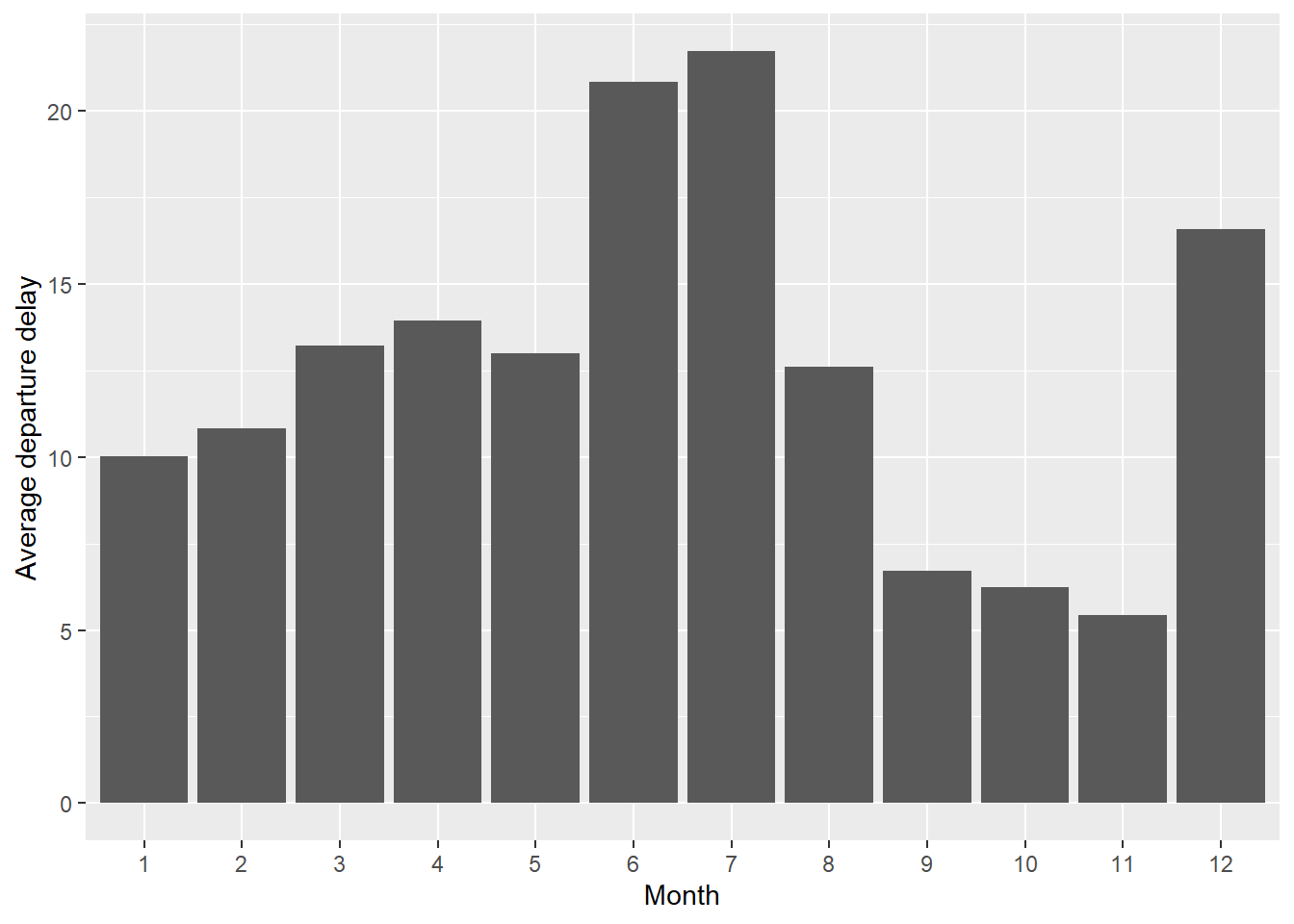
Notice the difference between %>% and + in the above code.

E.g. Create new columns for the average departure delay by date and average departure delay by destination using mutate

group_date <- group_by(select(flights, year:day, dep_delay, dest), month, day)
flights2 <- mutate(group_date, avg_date_dep_delay = mean(dep_delay, na.rm = TRUE))
group_dest <- group_by(flights2, dest)
(flights3 <- ungroup(mutate(group_dest, avg_dest_dep_delay = mean(dep_delay, na.rm = TRUE))))
## # A tibble: 336,776 × 7
##     year month   day dep_delay dest  avg_date_dep_delay avg_dest_dep_delay
##    <int> <int> <int>     <dbl> <chr>              <dbl>              <dbl>
##  1  2013     1     1         2 IAH                 11.5              10.8 
##  2  2013     1     1         4 IAH                 11.5              10.8 
##  3  2013     1     1         2 MIA                 11.5               8.88
##  4  2013     1     1        -1 BQN                 11.5              12.4 
##  5  2013     1     1        -6 ATL                 11.5              12.5 
##  6  2013     1     1        -4 ORD                 11.5              13.6 
##  7  2013     1     1        -5 FLL                 11.5              12.7 
##  8  2013     1     1        -3 IAD                 11.5              17.0 
##  9  2013     1     1        -3 MCO                 11.5              11.3 
## 10  2013     1     1        -2 ORD                 11.5              13.6 
## # ℹ 336,766 more rows

flights %>% 
  select(year:day, dep_delay, dest) %>% 
  group_by(month, day) %>% 
  mutate(avg_date_dep_delay = mean(dep_delay, na.rm = TRUE)) %>% 
  group_by(dest) %>% # By default, group_by() overrides existing grouping
  mutate(avg_dest_dep_delay = mean(dep_delay, na.rm = TRUE)) %>% 
  ungroup()
## # A tibble: 336,776 × 7
##     year month   day dep_delay dest  avg_date_dep_delay avg_dest_dep_delay
##    <int> <int> <int>     <dbl> <chr>              <dbl>              <dbl>
##  1  2013     1     1         2 IAH                 11.5              10.8 
##  2  2013     1     1         4 IAH                 11.5              10.8 
##  3  2013     1     1         2 MIA                 11.5               8.88
##  4  2013     1     1        -1 BQN                 11.5              12.4 
##  5  2013     1     1        -6 ATL                 11.5              12.5 
##  6  2013     1     1        -4 ORD                 11.5              13.6 
##  7  2013     1     1        -5 FLL                 11.5              12.7 
##  8  2013     1     1        -3 IAD                 11.5              17.0 
##  9  2013     1     1        -3 MCO                 11.5              11.3 
## 10  2013     1     1        -2 ORD                 11.5              13.6 
## # ℹ 336,766 more rows

4.11 Summary

Functions and operators learned in this chapter: arrange, filter, identical, %in%, tibble, ifelse, mutate, transmute, select, grep, group_by, summarize, ungroup, %>%

Chapter 4 Managing Data with R

4.1 Missing Values

4.2 Saving, loading, and removing R data structures

4.3 Importing and saving data from CSV files

4.4 Data Transformation with dplyr

4.5 arrange()